KdV: from a travelling wave to inverse scattering

A nonlinear wave can travel without spreading. That observation becomes much more powerful when the wave is encoded by a linear spectral problem whose data evolve simply. This sequence follows that connection for one Korteweg–de Vries (KdV) soliton: from a travelling-wave calculation to reflectionless scattering, reconstruction and a numerical convergence study.

You do not need to complete the Toda or spin-chain sequences first. The starting tools are differentiation, elementary differential equations and definite integration. The spectral and integral-equation calculations are developed as they are needed. Python and NumPy are required only to run the numerical laboratory; its method and selected results are readable without executing code.

The differential-equation bridge prepares solution checks, phase portraits and the care needed when separating an equation. Use it if those steps in the travelling-wave calculation are unfamiliar.

One pulse, two constructions

We use the real decaying-line equation

$$u_t+6u u_x+u_{xxx}=0,\qquad x\in\mathbb R.$$

The hyperbolic functions used below are $\operatorname{sech}z=2/(e^z+e^{-z})$ and $\tanh z=(e^z-e^{-z})/(e^z+e^{-z})$. In particular, $\operatorname{sech}z$ is positive, peaks at $z=0$, and decays at both ends of the line.

The positive pulse

$$u(x,t)=2\kappa^2\operatorname{sech}^2\!\left[\kappa(x-4\kappa^2t-x_0)\right], \qquad \kappa\gt0,$$

has peak height $2\kappa^2$, speed $4\kappa^2$ and inverse width $\kappa$. A taller pulse is narrower and faster. The parameter $x_0$ locates its center at $t=0$.

In the figure, compare the three widths at the initial time, then compare how far the centers move. Each curve is a separate exact solution; adding the curves would not give a solution of the nonlinear equation.

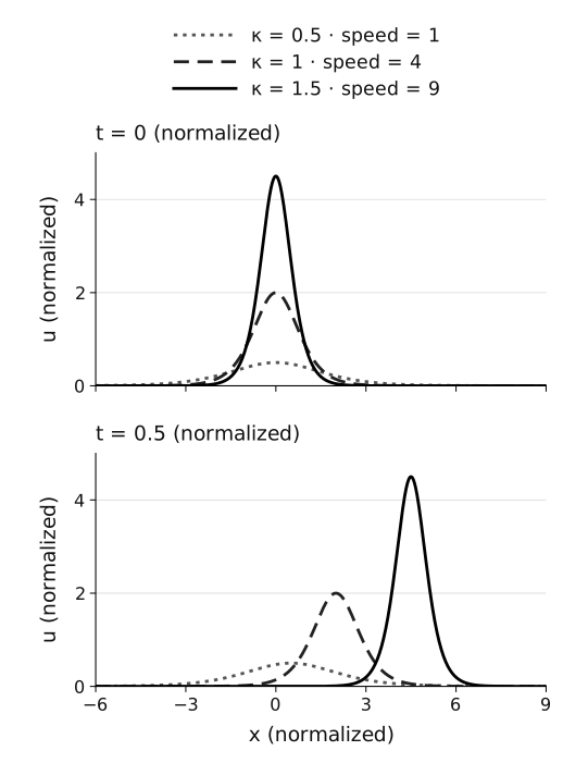
Amplitude, width and speed are linked in the KdV one-soliton family. The panels show exact profiles for $\kappa=0.5,1,1.5$, all with $x_0=0$, at normalized times $t=0$ and $t=0.5$. The panels share the same axes; these are three separate solutions, not a three-soliton collision.

$\kappa$	Peak height	Speed	Center at $t=0.5$
$0.5$	$0.5$	$1$	$0.5$
$1$	$2$	$4$	$2$
$1.5$	$4.5$	$9$	$4.5$

The first construction inserts a travelling profile into the nonlinear equation and uses decay to determine its shape. The second starts with one bound-state eigenvalue $-\kappa^2$ and a positive normalization constant, solves a linear integral equation, and recovers the same field. Matching the two fixes the meaning of the spectral data; it also exposes mistakes that a visually plausible pulse can conceal.

One explicit profile is not a proof that every initial condition has been solved. The model record defines the regime, and the Library article develops the operator calculation behind this example. The separate two-soliton follow-up shows how an exact collision changes the pulses’ positions. Broader initial data and general long-time asymptotics require additional theory.

Choose your starting point

Your question	Start here	What you should be able to do afterward
How can a nonlinear wave keep its shape?	Derive a travelling wave	Recover the amplitude, speed and width from an ODE and decay conditions
What prevents its integral quantities from changing?	Verify conservation laws	Identify the boundary terms in three conservation checks
Why does a Schrödinger equation enter a wave problem?	Relate the wave to scattering	Distinguish auxiliary eigenfunctions from the evolving physical field
How can spectral data reconstruct a wave?	Reconstruct one soliton	Solve the one-pole integral equation and interpret its normalization
How much numerical agreement is enough?	Run a convergence study	Separate time, space and finite-domain errors

For a first encounter, follow the order below. If you already have a capability, attempt that lesson’s independent exercise and move on when you can explain the solution without looking at the worked answer.

The seven-step sequence

1. Orient yourself here. Read the equation and distinguish the pulse from its auxiliary eigenfunction.
2. Derive the travelling wave. Reduce the PDE to an ODE, use the decay conditions, and determine the allowed pulse parameters.
3. Verify conserved integrals. Integrate by parts, keep the endpoint terms, and evaluate the results on the pulse.
4. Solve the auxiliary scattering problem. Identify the bound state and transmission amplitude of the pulse’s Schrödinger operator.
5. Reconstruct the pulse. Turn a single exponential kernel into an explicit solution and check the recovery sign.
6. Test numerical evolution. Compare computed motion with the exact profile while refining the step, resolution and domain independently.
7. Explain the two constructions. Match all parameters, reproduce selected checks and diagnose an intentionally inconsistent formula.

The laboratory and synthesis project have their own place in Practice & Projects, but the sequence links preserve this order. The later chapter map is a subject map, not an instruction to study every listed topic first.

Check your preparation

Before starting, try these three short calculations. They identify the tools used in the first lesson.

A moving profile. If $u(x,t)=U(x-vt)$, what are $u_t$ and $u_{xxx}$? What does a positive $v$ mean for the position of the maximum?

Check

The chain rule gives $u_t=-vU'$ and $u_{xxx}=U'''$, with derivatives taken in $z=x-vt$. A maximum initially at $z=z_0$ occurs at $x=z_0+vt$, so positive $v$ means motion to the right.

A boundary term. For a smooth decaying $f$, evaluate $\int_{\mathbb R}f f_x\,dx$ and explain the assumption you used.

Check

Since $f f_x=\tfrac12\partial_x(f^2)$, the integral is $\tfrac12[f^2]_{-\infty}^{+\infty}=0$, provided the integral exists and the endpoint values vanish. Merely naming “integration by parts” does not remove a nonzero boundary flux.

A decaying shape. Differentiate $\tanh z$, and use the result to integrate $\operatorname{sech}^2z$ over the line.

Check

$d(\tanh z)/dz=\operatorname{sech}^2z$. As $\tanh z$ tends to $1$ and $-1$ at the two ends, the integral is $2$. The identity $\operatorname{sech}^2z=1-\tanh^2z$ also converts the conserved-integral calculations into polynomial integrals on $[-1,1]$.

If a check is unfamiliar, work through its solution and the first lesson’s local preparation before proceeding. You need these particular tools, not an entire course in partial differential equations before meeting the example.

What the exit project establishes

By the end, you should be able to derive the pulse rather than recognize it, reconstruct it from stated spectral data, explain every convention conversion, and interpret a convergence table without confusing invariant preservation with small solution error. A useful final explanation includes the assumptions under which each calculation is valid.

To go beyond one travelling wave, measure a two-soliton collision, then verify its numerical evolution. This two-step follow-up distinguishes the asymptotic position shift from a peak measurement at finite time. The terminology reference explains what the collision adds to the solitary-wave example.

The open Toda sequence gives a finite matrix whose eigenvalues are conserved; KdV replaces it with a differential operator whose domain and asymptotic behavior matter. The XXX sequence instead uses scattering of physical spin excitations to build finite quantum eigenstates. The word “scattering” points to different objects in the two calculations. Comparing those objects is more informative than assuming that all exact methods have the same meaning.

For a quick formula translation use nonlinear-wave conventions. For checked source editions and downloads use the bibliography. References substantiate the course; its worked calculations and exercises are intended to make the chosen example self-contained.