Solve an oscillator two ways

Can changing coordinates turn an oscillation into uniform motion? For a classical harmonic oscillator, the answer is yes: its action stays fixed while its angle increases at a constant rate. You will obtain that description from the Hamiltonian, match the same initial position and momentum in both methods, and identify where the angle coordinate fails. The calculation concerns one undriven, undamped oscillator with positive mass and frequency.

Required background. Differentiate sine and cosine and use Hamilton’s equations. The Hamiltonian-bracket bridge explains the canonical bracket and how to test a change of coordinates.

Helpful background. The differential-equation bridge connects initial data to a phase portrait. The model record collects the physical parameters; the Liouville–Arnold reference places this explicit example within a theorem with stated hypotheses.

The oscillator and its initial data

Let $q\in\mathbb R$ be displacement, $p\in\mathbb R$ its conjugate momentum, $m\gt0$ the mass, and $\omega_0\gt0$ the angular frequency. On the phase plane use

$$H(q,p)=\frac{p^2}{2m}+\frac{m\omega_0^2q^2}{2}, \qquad \{f,g\}=f_qg_p-f_pg_q.$$

The initial conditions are arbitrary real numbers $q(0)=q_0$ and $p(0)=p_0$. The bracket gives

$$\dot q=\{q,H\}=\frac pm, \qquad \dot p=\{p,H\}=-m\omega_0^2q.$$

In particular, momentum is $m\dot q$. Energy is constant because $\dot H=\{H,H\}=0$. These are the Hamiltonian conventions of Cannas da Silva, January 2006 revision, § 18.2, p. 107, PDF. If using differential forms, they correspond to $\omega=dq\wedge dp$ and $\iota_{X_H}\omega=dH$; the frequency remains $\omega_0$.

Entry check and repair

Suppose $q(0)=a\gt0$ and $p(0)=0$. A proposed solution has $q(t)=a\cos(\omega_0t)$ and $p(t)=+m\omega_0a\sin(\omega_0t)$. Both initial values match. Is it a solution?

Repair. No: $m\dot q=-m\omega_0a\sin(\omega_0t)$, with the opposite sign. The force initially points toward the origin, so the momentum must become negative. Matching initial data is necessary, but the equations of motion must also hold. We will check both $q$ and $p$ in every representation.

First method: solve the differential equation

Differentiate $\dot q=p/m$ and use the second Hamilton equation:

$$\ddot q+\omega_0^2q=0.$$

Write its general solution as $q(t)=C\cos(\omega_0t)+D\sin(\omega_0t)$. The initial position gives $C=q_0$, and $m\dot q(0)=p_0$ gives $D=p_0/(m\omega_0)$. Hence

$$\boxed{ \begin{aligned} q(t)&=q_0\cos(\omega_0t)+\frac{p_0}{m\omega_0}\sin(\omega_0t),\\ p(t)&=p_0\cos(\omega_0t)-m\omega_0q_0\sin(\omega_0t). \end{aligned}}$$

Direct differentiation checks both Hamilton equations, and substituting $t=0$ checks both initial values. The conserved energy is

$$E=\frac{p_0^2}{2m}+\frac{m\omega_0^2q_0^2}{2}.$$

At $E\gt0$, the orbit is an ellipse in the $(q,p)$ plane. The displacement amplitude and period are

$$A=\sqrt{q_0^2+\left(\frac{p_0}{m\omega_0}\right)^2}, \qquad T=\frac{2\pi}{\omega_0}.$$

The amplitude depends on the initial data; the period does not. The exact formula also covers $E=0$, when $q(t)=p(t)=0$.

Second method: construct the action and angle

For $E\gt0$, define

$$I=\frac H{\omega_0} =\frac{p^2}{2m\omega_0}+\frac{m\omega_0q^2}{2}\gt0$$

and parameterize the ellipse by

$$\boxed{ q=\sqrt{\frac{2I}{m\omega_0}}\sin\theta, \qquad p=\sqrt{2m\omega_0I}\cos\theta.}$$

Here $\theta$ is an angle modulo $2\pi$. With $q$ horizontal and $p$ vertical, $\theta=0$ is the top of the ellipse. Increasing $\theta$ moves rightward from there, following the clockwise physical motion.

The action is more than a rescaled energy: it measures an oriented phase-space area. Traverse a positive-energy orbit once in the direction of increasing physical time. Since $I$ is fixed on this cycle,

$$\begin{aligned} \frac1{2\pi}\oint p\,dq &=\frac1{2\pi}\int_0^{2\pi}2I\cos^2\theta\,d\theta\\ &=I=\frac E{\omega_0}. \end{aligned}$$

The integral is positive for this orientation. Reversing the cycle reverses its sign. In Torrielli 2016, § 2.2, pp. 6–7, equations (2.18) and (2.23)–(2.32), v1 PDF, the unit-mass, unit-frequency oscillator is instead parameterized counterclockwise by $q=R\cos\alpha$, $p=R\sin\alpha$. His chosen cycle gives $I_{\mathrm T}=-E$. Our variables are related by $I=-I_{\mathrm T}$ and $\theta=\pi/2-\alpha$ modulo $2\pi$ at those units. The orientation and angle are changed together.

The figure makes the angle orientation visible. Choose a fixed action scale $I_*\gt0$ and use dimensionless coordinates

$$X=\sqrt{\frac{m\omega_0}{2I_*}}\,q, \qquad Y=\frac{p}{\sqrt{2m\omega_0I_*}}.$$

Then $X^2+Y^2=I/I_*$, $\dot X=\omega_0Y$ and $\dot Y=-\omega_0X$. Follow the clockwise arrows from the positive $Y$ axis; the center belongs to no positive-action orbit.

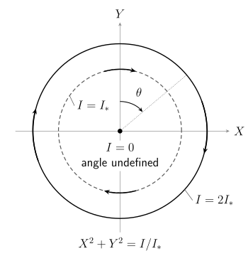
Exact phase curves in the normalized $(X,Y)$ plane for $m,\omega_0,I_*\gt0$. The dashed orbit has $I=I_*$ and radius $1$; the solid orbit has $I=2I_*$ and radius $\sqrt2$. Both advance with $\dot\theta=\omega_0$, while the origin is stationary and its angle is undefined. Arrow lengths do not encode speed.

Check the canonical bracket

Drawing an ellipse does not prove that its parameters are canonical. On any smooth local branch of the angle, write

$$\theta=\operatorname{atan2}(m\omega_0q,p), \qquad D=p^2+m^2\omega_0^2q^2\gt0.$$

Our notation $\operatorname{atan2}(Y,X)$ means the quadrant-aware angle whose sine and cosine are proportional to $Y$ and $X$, respectively. The two arguments here have the same momentum units. Differentiation on a branch gives

$$\begin{aligned} \theta_q&=\frac{m\omega_0p}{D}, &\theta_p&=-\frac{m\omega_0q}{D},\\ I_q&=m\omega_0q, &I_p&=\frac p{m\omega_0}. \end{aligned}$$

Therefore

$$\{\theta,I\} =\theta_qI_p-\theta_pI_q =\frac{p^2+m^2\omega_0^2q^2}{D}=1.$$

Equivalently, substitution gives $dq\wedge dp=d\theta\wedge dI$. Thus $\theta$ is the new coordinate and $I$ its conjugate momentum. The Hamiltonian becomes

$$H=\omega_0 I, \qquad \dot I=-\frac{\partial H}{\partial\theta}=0, \qquad \dot\theta=\frac{\partial H}{\partial I}=\omega_0.$$

Integration now yields $I(t)=I_0$ and $\theta(t)=\theta_0+\omega_0t$ modulo $2\pi$. The nonlinear change of coordinates has converted the elliptical motion into uniform angular motion.

Match the same position and momentum

For nonzero initial data, the matching constants are

$$\begin{aligned} I_0&=\frac{p_0^2}{2m\omega_0}+\frac{m\omega_0q_0^2}{2},\\ \theta_0&=\operatorname{atan2}(m\omega_0q_0,p_0)\pmod{2\pi}. \end{aligned}$$

In particular,

$$\sin\theta_0=\frac{q_0}{A}, \qquad \cos\theta_0=\frac{p_0}{m\omega_0A}.$$

Both relations matter. An inverse sine alone cannot distinguish the sign of momentum, and a one-argument inverse tangent loses the quadrant.

Substitute $\theta_0+\omega_0t$ into the position formula and use the sine addition rule:

$$\begin{aligned} q(t)&=A\sin\theta_0\cos(\omega_0t) +A\cos\theta_0\sin(\omega_0t)\\ &=q_0\cos(\omega_0t)+\frac{p_0}{m\omega_0}\sin(\omega_0t). \end{aligned}$$

The cosine addition rule similarly gives

$$\begin{aligned} p(t)&=m\omega_0A\cos\theta_0\cos(\omega_0t) -m\omega_0A\sin\theta_0\sin(\omega_0t)\\ &=p_0\cos(\omega_0t)-m\omega_0q_0\sin(\omega_0t). \end{aligned}$$

The two methods now produce exactly the same trajectory, including the momentum and its sign.

A quadrant-sensitive example

Take $q_0=a\gt0$ and $p_0=-m\omega_0a$. Then

$$A=\sqrt2a, \qquad I_0=m\omega_0a^2, \qquad \theta_0=\frac{3\pi}{4}.$$

The solution is

$$\begin{aligned} q(t)&=a\bigl[\cos(\omega_0t)-\sin(\omega_0t)\bigr],\\ p(t)&=-m\omega_0a\bigl[\cos(\omega_0t)+\sin(\omega_0t)\bigr]. \end{aligned}$$

Using $\theta_0=\pi/4$ would reproduce the initial position but reverse the initial momentum. At $t=\pi/(4\omega_0)$ the correct trajectory crosses $q=0$ with $p=-\sqrt2m\omega_0a$, giving a further direction check.

Dimensions and the missing angle at equilibrium

If $q$ has units of length, then $p$ has units of momentum and $I$ has units of energy times time, or action. The angle is dimensionless and measured in radians. Consequently $H=\omega_0I$ has energy units and $\dot\theta=\omega_0$ has inverse-time units. There is no quantization assumption: every real $I\geq0$ occurs in this classical model.

At $I=0$, the ellipse collapses to the equilibrium $(q,p)=(0,0)$. Every angle in the parameterization gives the same point, so the angle cannot be recovered and the change of coordinates is not invertible there. This is a coordinate singularity, not a divergent physical solution.

Even away from the origin, a single real-valued angle cannot be continuous around a complete cycle: following the cycle once increases a lifted angle by $2\pi$. The punctured phase plane is globally parameterized by $(I,\theta)\in(0,\infty)\times(\mathbb R/2\pi\mathbb Z)$, while a real-valued branch of $\theta$ uses a cut. Along one chosen trajectory, an unwrapped real angle can be continued for all time.

Positive-energy ellipses are compact, connected regular levels of $H$; the origin has $dH=0$ and is not a regular level. This is the simplest setting for the compact-torus conclusion of Cannas da Silva, § 18.4, pp. 110–111, Lemma 18.11 and Theorem 18.12, PDF. The theorem reference explains why its local action–angle conclusion does not supply one real coordinate chart through all equilibria and all cycles.

Exercises

Guided practice: start at a turning point

Let $q_0=a\gt0$ and $p_0=0$. Determine $I_0$ and $\theta_0$, write the direct and action–angle solutions, and compute $(q,p)$ after one quarter-period. Check the sign of the momentum.

Hint

The initial sine is positive and the initial cosine is zero. Use $T=2\pi/\omega_0$ and advance the angle by $\pi/2$ during $T/4$.

Solution

The constants are $I_0=m\omega_0a^2/2$ and $\theta_0=\pi/2$ modulo $2\pi$. Thus

$$\begin{aligned} q(t)&=a\sin(\pi/2+\omega_0t)=a\cos(\omega_0t),\\ p(t)&=m\omega_0a\cos(\pi/2+\omega_0t) =-m\omega_0a\sin(\omega_0t). \end{aligned}$$

At $T/4$, $(q,p)=(0,-m\omega_0a)$. The particle has moved from the positive turning point toward the origin, so negative momentum is required. Its energy remains $m\omega_0^2a^2/2$.

Independent practice: recover the quadrant

For $a\gt0$, take $q_0=-a$ and $p_0=-\sqrt3m\omega_0a$. Find the energy $E$, amplitude $A$, initial action $I_0$, and phase $\theta_0\in[0,2\pi)$. Produce both solution forms and their quarter-period values. Explain why using only $\arctan(m\omega_0q_0/p_0)$ gives the wrong initial state.

Hint

Both sine and cosine must be negative. After finding $A$, calculate their individual values before selecting an angle.

Solution

The energy is $E=2m\omega_0^2a^2$, so $A=2a$ and $I_0=2m\omega_0a^2$. The sine and cosine are $-1/2$ and $-\sqrt3/2$, giving $\theta_0=7\pi/6$. With $s=\omega_0t$,

$$\begin{aligned} q(t)&=2a\sin(s+7\pi/6) =-a\cos s-\sqrt3a\sin s,\\ p(t)&=2m\omega_0a\cos(s+7\pi/6)\\ &=-\sqrt3m\omega_0a\cos s+m\omega_0a\sin s. \end{aligned}$$

At $T/4$, the state is $(-\sqrt3a,m\omega_0a)$. The one-argument arctangent instead returns $\pi/6$, because the ratio is $1/\sqrt3$; that phase reverses both initial signs. Checking $q(0)$ and $p(0)$ independently exposes the error.

Transfer: let the restoring frequency vanish

Keep $m,q_0,p_0$ and a finite observation time $t$ fixed, with $p_0\ne0$, and let $\omega_0\to0^+$. Find the limit of the direct solution. What happens to $I_0$ and $T$? Explain why substituting $\omega_0=0$ into the action–angle formulas is invalid even though the physical limit exists.

Hint

Use $\sin(\omega_0t)/\omega_0\to t$. Compare the positive-energy level sets of $p^2/(2m)$ with the ellipses of a positive-frequency oscillator.

Solution

The limiting solution is free motion:

$$q(t)\longrightarrow q_0+\frac{p_0}{m}t, \qquad p(t)\longrightarrow p_0.$$

Meanwhile

$$I_0=\frac{p_0^2}{2m\omega_0}+\frac{m\omega_0q_0^2}{2} \longrightarrow\infty, \qquad T=\frac{2\pi}{\omega_0}\longrightarrow\infty.$$

At zero frequency, each connected positive-energy level is a noncompact line with constant nonzero momentum. There is no closed orbit over which to define this oscillator action. The transformation degenerates although the direct solution has a regular fixed-time limit. This limit is not uniform over times that grow like $1/\omega_0$. If $p_0=0$, the fixed-time limit is stationary instead, and the stated divergence of $I_0$ does not apply.

Use the example beyond the oscillator

The calculation has established an explicit canonical transformation on the punctured phase plane, uniform angle evolution, and agreement with arbitrary initial data. Its failures at the equilibrium and at zero restoring frequency illustrate why regularity and compactness belong in an action–angle theorem. Continue with Build actions and angles to derive a nonlinear oscillator’s energy-dependent frequency, the Liouville–Arnold reference for the theorem’s hypotheses, or the open Toda sequence to study an interacting system.

References

• Cannas da Silva, Ana. Lectures on Symplectic Geometry. Lecture Notes in Mathematics 1764, Springer, 2001. DOI. Author revision January 2006; MIT-hosted PDF. Locators above use the printed pages of this revision.
• Torrielli, Alessandro. Lectures on Classical Integrability. arXiv:1606.02946v1 [hep-th], 2016. Version record. Open PDF. The action-cycle orientation is translated explicitly above.