Measure a KdV soliton collision

What remains unchanged when two KdV solitons collide, and what changes? Far before and after the interaction, each pulse has the same amplitude and speed, but its outgoing trajectory is displaced from its incoming trajectory. You will extract those straight lines from an exact two-soliton solution, calculate the advance of the faster pulse and the delay of the slower one, and explain why simply adding two travelling waves misses the collision.

Required background. Derive a KdV travelling wave establishes the single-pulse profile and its amplitude–speed relation. You will also use exponentials, logarithms and partial derivatives.

Helpful background. Reconstruct a one-soliton solution introduces $u=2\partial_x^2\log\tau$. The solitary-wave and soliton reference explains the distinction that this collision makes concrete.

Two distinct solitons in one exact field

Use the positive-pulse convention

$$u_t+6uu_x+u_{xxx}=0,\qquad x,t\in\mathbb R,$$

with a real smooth field decaying as $x\to\pm\infty$ at each fixed time. Choose two distinct inverse widths and two real phase parameters:

$$\kappa_1\gt\kappa_2\gt0,\qquad x_1,x_2\in\mathbb R.$$

Define

$$\begin{aligned} \eta_j&=2\kappa_j(x-4\kappa_j^2t-x_j),\qquad j=1,2,\\ A&=\left(\frac{\kappa_1-\kappa_2}{\kappa_1+\kappa_2}\right)^2,\\ \tau&=1+e^{\eta_1}+e^{\eta_2}+Ae^{\eta_1+\eta_2}. \end{aligned}$$

The exact two-soliton field is

$$u(x,t)=2\partial_x^2\log\tau =2\frac{\tau\tau_{xx}-\tau_x^2}{\tau^2}.$$

Since $0\lt A\lt1$, all four terms in $\tau$ are positive, so its logarithm has no singularity. As $x\to-\infty$, $\tau\to1$; as $x\to+\infty$, the last exponential dominates. In either case the second logarithmic derivative decays. The full field, rather than a sum of independently prescribed pulses, supplies the initial condition at any chosen time.

The finite-rank reconstruction behind this expression is Aktosun 2009, § IX, equations (9.1)–(9.3). His KdV field has the opposite sign: writing it as $q=-u$ converts his $q_t-6qq_x+q_{xxx}=0$ to our equation. The Library derivation obtains the two-by-two determinant, translates its phase parameters, and checks the PDE. Here the task is to read the collision from the resulting scalar function.

The labels $1$ and $2$ follow the parameters $\kappa_j$: soliton $1$ is faster because $4\kappa_1^2\gt4\kappa_2^2$. They do not mean “left peak” and “right peak” at every time. Also, $x_1,x_2$ are phase parameters; they are not both incoming center intercepts.

Entry check: which factors move a pulse?

Let $\widetilde\tau=e^{ax+bt+d}\tau$, with real constants $a,b,d$. Does $2\partial_x^2\log\widetilde\tau$ give the same field? Does this allow you to discard a positive coefficient $C$ inside $1+Ce^\eta$?

Repair: separate an overall factor from a relative coefficient

The logarithm of the overall factor is $ax+bt+d$, whose second $x$ derivative is zero. Thus multiplying the entire tau function by this factor leaves $u$ unchanged. In contrast, $1+Ce^\eta$ changes the relative size of its two terms:

$$1+Ce^\eta=1+e^{\eta+\log C}.$$

The coefficient shifts the phase and therefore the pulse center. It cannot be dropped unless the corresponding position shift is retained.

Read a center from a surviving exponential

For $C\gt0$ and $\eta=2\kappa(x-4\kappa^2t-x_0)$, direct differentiation gives

$$\begin{aligned} 2\partial_x^2\log(1+Ce^\eta) &=\frac{8\kappa^2Ce^\eta}{(1+Ce^\eta)^2}\\ &=2\kappa^2\operatorname{sech}^2 \left(\frac{\eta+\log C}{2}\right). \end{aligned}$$

Its maximum occurs when $\eta+\log C=0$, so its center is

$$X(t)=4\kappa^2t+x_0-\frac{\log C}{2\kappa}.$$

The coefficient $C$ changes the intercept. The amplitude $2\kappa^2$, speed $4\kappa^2$ and width scale $1/\kappa$ stay fixed. In particular, $C=A\lt1$ shifts the center to the right because $\log A\lt0$.

To apply this observation to a collision, follow one pulse as time grows in magnitude. Taking $t\to\pm\infty$ at a fixed laboratory position would miss both right-moving pulses. Instead, hold a coordinate moving at the chosen soliton’s speed fixed.

Follow the fast pulse through both time limits

Set

$$\xi_1=x-4\kappa_1^2t-x_1.$$

At fixed $\xi_1$, the first phase is $\eta_1=2\kappa_1\xi_1$, while

$$\eta_2=2\kappa_2\left[ 4(\kappa_1^2-\kappa_2^2)t+x_1-x_2+\xi_1 \right].$$

The coefficient of $t$ is positive. Therefore, as $t\to-\infty$, $e^{\eta_2}\to0$ and

$$\tau\longrightarrow1+e^{\eta_1}.$$

The incoming fast-pulse center approaches the line $4\kappa_1^2t+x_1$.

As $t\to+\infty$, $e^{\eta_2}$ grows. Factor it out before taking the limit:

$$\frac{\tau}{e^{\eta_2}} =e^{-\eta_2}(1+e^{\eta_1})+1+Ae^{\eta_1} \longrightarrow1+Ae^{\eta_1}.$$

The factor $e^{\eta_2}$ contributes nothing to the second logarithmic derivative. The outgoing fast-pulse line is consequently

$$4\kappa_1^2t+x_1-\frac{\log A}{2\kappa_1}.$$

For fixed distinct $\kappa_j$, the discarded terms and their first two spatial derivatives tend to zero exponentially on each bounded $\xi_1$ interval. This justifies extracting the limiting profile after differentiating the logarithm; it is more than a comparison of the largest terms in $\tau$.

Follow the slow pulse and compare the lines

Now hold $\xi_2=x-4\kappa_2^2t-x_2$ fixed. Then

$$\eta_1=2\kappa_1\left[ 4(\kappa_2^2-\kappa_1^2)t+x_2-x_1+\xi_2 \right].$$

This time the coefficient of $t$ is negative. At early times $\eta_1\to+\infty$, and

$$\frac{\tau}{e^{\eta_1}} =e^{-\eta_1}(1+e^{\eta_2})+1+Ae^{\eta_2} \longrightarrow1+Ae^{\eta_2}.$$

At late times $\eta_1\to-\infty$ and $\tau\to1+e^{\eta_2}$. The slow pulse therefore carries the coefficient $A$ before the collision, whereas the fast pulse carries it after the collision.

Write each asymptotic line as

$$X_j^\pm(t)=4\kappa_j^2t+b_j^\pm,$$

where $-$ labels incoming and $+$ outgoing. The calculation gives

Soliton	Incoming intercept $b_j^-$	Outgoing intercept $b_j^+$
Fast, $j=1$	$x_1$	$x_1-\log A/(2\kappa_1)$
Slow, $j=2$	$x_2-\log A/(2\kappa_2)$	$x_2$

Define the signed position shift by comparing these intercepts, or equivalently by comparing the two extrapolated lines at the same time:

$$\begin{aligned} \Delta X_1&=b_1^+-b_1^- =-\frac{\log A}{2\kappa_1}\gt0,\\ \Delta X_2&=b_2^+-b_2^- =\frac{\log A}{2\kappa_2}\lt0. \end{aligned}$$

The fast soliton advances; the slow one lags. Their shifts are independent of $x_1,x_2$, which set where and when the interaction occurs. A useful sign and normalization check is

$$\kappa_1\Delta X_1+\kappa_2\Delta X_2=0.$$

An advance does not mean that the outgoing fast pulse has a permanently larger speed: the two lines have the same slope. A position shift is also different from subtracting the pulse’s positions at two different times, which includes ordinary travel.

A collision with explicit intercepts

Use nondimensional values $\kappa_1=1$, $\kappa_2=1/2$, so $A=1/9$. Choose

$$x_1=-\frac{\log3}{2},\qquad x_2=-\log3.$$

These phases give the following asymptotic data:

Quantity	Fast soliton	Slow soliton
Amplitude, before and after	$2$	$1/2$
Speed, before and after	$4$	$1$
Incoming line	$4t-\log3/2$	$t+\log3$
Outgoing line	$4t+\log3/2$	$t-\log3$
Signed position shift	$\log3$	$-2\log3$

For example, the slow incoming intercept is $x_2-\log(1/9)=\log3$, not the phase parameter $x_2=-\log3$. Both shifts follow from one exact field.

The three profiles below show what happens between those separated limits. At $t=0$, the phases give the independent check

$$\tau(x,0)=(1+e^x)^3, \qquad u(x,0)=\frac32\operatorname{sech}^2(x/2).$$

The overlap peak has height $3/2$, which differs from both separated amplitudes $2$ and $1/2$.

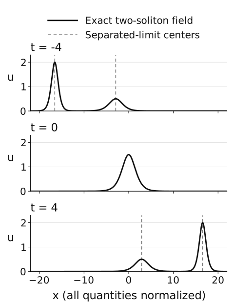
One exact field at $t=-4,0,4$, with the parameters above and shared linear axes. Dashed vertical lines mark the extrapolated incoming centers at $t=-4$ and outgoing centers at $t=4$; they are asymptotic predictions, not exact finite-time maxima. No individual pulse centers are assigned during overlap. The plot uses the exact tau function, not a numerical PDE evolution.

“Before and after” means the separated limits, not every moment of overlap. During the collision the field is deformed, and two distinct local maxima need not persist. Matching the solitons by their asymptotic speeds avoids assigning a physical identity to a peak through an ambiguous merger. The result establishes elastic two-soliton scattering in this exact family; it is not a claim that arbitrary initial waves have no radiation.

Why the sum of two pulses is not exact

Let $u_1,u_2$ be two exact single-pulse solutions and define the KdV residual of a field $w$ by

$$\mathcal R[w]=w_t+6ww_x+w_{xxx}.$$

Expanding the nonlinear term and using $\mathcal R[u_1]=\mathcal R[u_2]=0$ yields

$$\mathcal R[u_1+u_2] =6(u_1u_{2x}+u_2u_{1x}) =6\partial_x(u_1u_2).$$

Their product is positive at finite positions and tends to zero at spatial infinity, so it is not constant; its derivative cannot vanish identically. Thus the sum fails the PDE, even though its residual may vanish at particular points. When the pulses are far apart, overlap is exponentially small and the sum is a useful approximation. Through the interaction, use the full tau function.

The collision laboratory tests a numerical evolution against this exact solution. At finite observation times, measured centers have remaining interaction corrections as well as discretization error. Increasing pulse separation and refining the computation answer different questions.

Exercises

Guided: calculate the advance and lag

Take $\kappa_1=3/2$, $\kappa_2=1/2$ and $x_1=x_2=0$. Compute $A$, all four intercepts, both position shifts, and the two amplitudes and speeds. Check the weighted-shift identity.

Hint

Here $(\kappa_1-\kappa_2)/(\kappa_1+\kappa_2)=1/2$. Insert the resulting $\log A$ into the intercept table before subtracting.

Solution

We have $A=1/4$ and $\log A=-2\log2$. Hence

$$\begin{aligned} b_1^-&=0,& b_1^+&=\frac23\log2,\\ b_2^-&=2\log2,& b_2^+&=0. \end{aligned}$$

The shifts are $\Delta X_1=(2/3)\log2$ and $\Delta X_2=-2\log2$. Their weighted sum is

$$\frac32\left(\frac23\log2\right) +\frac12(-2\log2)=0.$$

The amplitudes are $9/2$ and $1/2$; the speeds are $9$ and $1$. Each pair of incoming and outgoing lines has the same slope. The larger negative shift belongs to the slower pulse, but both pulses still move to the right.

Independent: prescribe the incoming trajectories

For $\kappa_1=1$ and $\kappa_2=1/2$, prescribe the incoming lines $4t-5$ and $t+2$. Find the phase parameters $x_1,x_2$ to use in $\tau$, then predict both outgoing lines. Explain the error in setting $x_2=2$.

Hint

Solve $b_1^-=x_1$ and $b_2^-=x_2-\log A/(2\kappa_2)$ for the phase parameters. This is an inverse use of the table.

Solution

Since $A=1/9$, the phases are

$$x_1=-5,\qquad x_2=2-2\log3.$$

The outgoing lines are

$$X_1^+(t)=4t-5+\log3, \qquad X_2^+(t)=t+2-2\log3.$$

Setting $x_2=2$ would prescribe the slow incoming line $t+2+2\log3$, not the requested $t+2$. The phase shifts would remain the same, but the initial arrangement and collision location would differ.

Transfer: let the two inverse widths approach each other

Keep $x_1=x_2=0$ and let $\kappa_1,\kappa_2\to\kappa\gt0$ through $\kappa_1\gt\kappa_2$. What happens to $A$ and the shift formulas? Separately take the limit of $\tau$ at fixed finite $x,t$. Identify the resulting field. Why is this not a collision of two distinct equal-speed pulses with infinite shifts?

Hint

At fixed $x,t$, both phases tend to $\eta=2\kappa(x-4\kappa^2t)$. Retain the coefficient of $e^\eta$ when applying the single-exponential formula. Compare this limit with the moving-frame time limits used earlier.

Solution

Here $A\to0$ and $\log A\to-\infty$, so $\Delta X_1\to+\infty$ and $\Delta X_2\to-\infty$. But at fixed finite $x,t$,

$$\tau\longrightarrow1+2e^\eta.$$

The same limit holds after the needed spatial differentiations on bounded space-time sets. Consequently,

$$u\longrightarrow2\kappa^2\operatorname{sech}^2 \left[\kappa(x-4\kappa^2t)+\frac{\log2}{2}\right].$$

This is one pulse, centered at $4\kappa^2t-\log2/(2\kappa)$. The distinct-pulse asymptotics assumed fixed $\kappa_1\gt\kappa_2$ before sending $t\to\pm\infty$. As their difference shrinks, the relative speed $4(\kappa_1^2-\kappa_2^2)$ vanishes and those limits cease to be uniform in the parameters. Interchanging them changes the question. This limiting calculation does not construct a two-pulse equal-speed scattering process.

From exact shifts to a numerical measurement

You can now obtain each incoming and outgoing line by choosing a moving frame, removing an irrelevant overall exponential, and keeping the coefficient of the surviving phase. Continue to measure a collision numerically using the full exact solution as the benchmark. For the reconstruction and PDE proof supporting the formula, use two-soliton scattering in the Library.

References

• Aktosun, Tuncay. “Inverse Scattering Transform and the Theory of Solitons.” In Encyclopedia of Complexity and Systems Science, edited by Robert A. Meyers, pp. 4960–4971. Springer, 2009. DOI. Author version arXiv:0905.4746v1, § IX, equations (9.1)–(9.3); open text, PDF.