Build actions and angles

Can a nonlinear oscillator have a uniformly advancing angle? Yes, although different energy curves generally have different angular frequencies. For the quartic oscillator, the action is proportional to $E^{3/4}$ and the frequency to $E^{1/4}$. You will derive both laws, construct the angle from elapsed physical time, and continue it through the turning points. The result applies to every positive-energy orbit of this one-degree-of-freedom system; the equilibrium requires separate treatment.

Required background. The Hamiltonian bridge supplies Hamilton’s equations, the canonical bracket and the chain rule. You need definite integrals and partial derivatives. Helpful background. What makes a system integrable? introduces this quartic energy curve. Solve an oscillator two ways constructs harmonic action–angle coordinates, whose constant frequency provides a comparison.

A quartic energy curve and its orientation

Work on the real phase space $(q,p)\in\mathbb R^2$ with real time $t\in\mathbb R$, all made dimensionless by fixed scales. Use

$$H(q,p)=\frac{p^2}{2}+\frac{q^4}{4},\qquad \{f,g\}=f_qg_p-f_pg_q.$$

Thus $\dot q=p$, $\dot p=-q^3$ and $\dot H=0$. At energy $E\gt0$, put

$$a=(4E)^{1/4},\qquad p_+(q;E)=\sqrt{2E-q^4/2},\qquad |q|\le a.$$

The upper branch has $p=p_+\gt0$ and moves right; the lower branch has $p=-p_+$ and moves left. Together they form a compact regular closed orbit. The existing quartic phase portrait shows this motion. Traversing it in physical time makes $\oint p\,dq$ positive: both $p$ and $dq$ reverse sign on the lower branch.

All quantities here are dimensionless after the stated scaling. With dimensional coordinates, an action has the units of momentum times position, and an energy derivative with respect to action has units of angular frequency.

Entry check: conservation does not fix an angle

Since $H$ is conserved, someone proposes $I=H$ and the ordinary polar angle $\phi=\operatorname{atan2}(q,p)$, measured clockwise from the positive $p$ axis. Does conservation alone make this pair canonical with a uniformly advancing angle?

Check and repair

On a real branch away from the origin,

$$\{\phi,H\}=\frac{p^2+q^4}{p^2+q^2}.$$

This is neither identically one nor constant along a positive-energy curve. For example, on $E=1/4$ it is one at $q=0$, but $17/23$ at $q=1/2$. A conserved first coordinate is insufficient: we must check the canonical bracket and the angle’s period. The correct angle will measure elapsed time, rather than geometric polar direction.

Integrate the positive action

Define the action using one primitive cycle—one full circuit—in the direction of physical flow:

$$I(E)=\frac1{2\pi}\oint p\,dq =\frac2\pi\int_0^a\sqrt{2E-q^4/2}\,dq.$$

The factor four in the closed integral accounts for all four quarter-orbits. Substitute $q=ar$, using $a\sqrt{2E}=2E^{3/4}$:

$$I(E)=\frac4\pi E^{3/4}\int_0^1\sqrt{1-r^4}\,dr.$$

The remaining constant is a beta integral. For positive real $x,y$, define

$$\mathrm B(x,y)=\int_0^1z^{x-1}(1-z)^{y-1}\,dz.$$

Setting $z=r^4$ gives $dr=\tfrac14z^{-3/4}dz$, so

$$I(E)=CE^{3/4},\qquad C=\frac{\mathrm B(1/4,3/2)}{\pi}\gt0.$$

This special-function notation names a definite positive constant; no beta-function theory is needed to follow the substitution. The definition and identity $\mathrm B(x,y)=\Gamma(x)\Gamma(y)/\Gamma(x+y)$ are DLMF, equation (5.12.1). Together with $\Gamma(z+1)=z\Gamma(z)$ from DLMF, equation (5.5.1), they give

$$\mathrm B(1/4,3/2)=\frac23\mathrm B(1/4,1/2), \qquad C=\frac{2\mathrm B(1/4,1/2)}{3\pi}.$$

The cycle definition follows the action construction in Torrielli 2016, §2.2, printed p. 6, equation (2.18), v1 PDF. His harmonic example traverses its cycle in the opposite orientation, giving a negative action in equation (2.31). We follow physical time and choose the positive action, as in the site’s harmonic lesson; orientation and angle direction must be translated together.

Differentiate the action to obtain the period

Since $\dot q=p_+$ on the outgoing quarter-orbit,

$$\begin{aligned} T(E)&=4\int_0^a\frac{dq}{\sqrt{2E-q^4/2}}\\ &=4E^{-1/4}\int_0^1\frac{dr}{\sqrt{1-r^4}}\\ &=\mathrm B(1/4,1/2)E^{-1/4}. \end{aligned}$$

The integrable square-root endpoint gives a finite period at every $E\gt0$. Differentiating $I=CE^{3/4}$ and using the beta identity yields

$$\boxed{\frac{dI}{dE}=\frac{T(E)}{2\pi}.}$$

There is also a direct reason for this relation. Differentiating the action integrand gives $\partial p_+/\partial E=1/p_+$. The moving endpoint contributes zero because $p_+(a;E)=0$, and the derivative’s inverse-square-root endpoint is integrable. Thus

$$\frac{dI}{dE}=\frac2\pi\int_0^a\frac{dq}{p_+(q;E)} =\frac{T(E)}{2\pi}.$$

The fixed-interval substitution above also justifies this differentiation without relying on a formal endpoint cancellation.

Because $I(E)$ is strictly increasing, we can invert it:

$$H(I)=\left(\frac IC\right)^{4/3},\qquad \Omega(I)=\frac{dH}{dI} =\frac4{3C}\left(\frac IC\right)^{1/3}.$$

Equivalently, at energy $E$,

$$\Omega(I(E))=\frac{2\pi}{T(E)} =\frac{2\pi E^{1/4}}{\mathrm B(1/4,1/2)}.$$

Each orbit has a constant frequency, but the family of orbits does not share one frequency. Increasing the action by a factor eight doubles the frequency. If $I_*=I(1/4)$ and $\Omega_*=\Omega(I_*)$, the exact comparison is

$$\frac{\Omega(I)}{\Omega_*}=\left(\frac I{I_*}\right)^{1/3}.$$

A harmonic oscillator chosen to have frequency $\Omega_*$ instead has $\Omega/\Omega_*=1$ at every positive action. This compares two different Hamiltonians; it is not a harmonic approximation to the quartic oscillator near its origin.

The figure compares the exact frequency laws and marks the eightfold-action scaling.

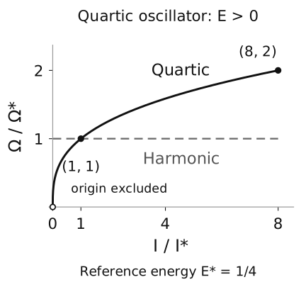
Exact normalized frequencies for positive action. The quartic curve uses $I_*=I(E_*=1/4)$ and $\Omega_*=\Omega(I_*)$: increasing action eightfold doubles frequency. The dashed harmonic comparison has frequency $\Omega_*$, without an equal-energy requirement. The open origin indicates the excluded quartic equilibrium limit.

Construct a canonical angle on one branch

Choose the crossing $q=0,p\gt0$ as angle zero. On the open upper branch, $|q|\lt a(H(I))$, define the generating function

$$W(q,I)=\int_0^q\sqrt{2H(I)-s^4/2}\,ds.$$

It satisfies $W_q=p_+$. Define the local angle by

$$\begin{aligned} \Theta(q,I)&=\frac{\partial W}{\partial I}\\ &=\Omega(I)\int_0^q\frac{ds}{\sqrt{2H(I)-s^4/2}}. \end{aligned}$$

The integral is signed elapsed time from the chosen crossing along the upper branch. The generating-function prescription and the angle’s $2\pi$ change around a cycle are developed in Torrielli 2016, §2.2, printed p. 6, equations (2.19)–(2.22), v1 PDF. Here we check the local bracket explicitly.

Set $\theta(q,p)=\Theta(q,I(H(q,p)))$ on $p\gt0$. Holding $I$ fixed,

$$\left.\frac{\partial\Theta}{\partial q}\right|_I=\frac{\Omega}{p}, \qquad \left.\frac{\partial I}{\partial p}\right|_q =\frac{dI}{dE}p=\frac p\Omega.$$

In the chain rule for $\{\theta,I\}$, the two terms containing $\Theta_I$ cancel. Therefore

$$\boxed{\{\theta,I\} =\left.\Theta_q\right|_I\left.I_p\right|_q=1.}$$

Consequently $\dot I=0$ and $\dot\theta=\{\theta,H(I)\}=\Omega(I)$. This proves canonicity and uniform advance on the branch, rather than inferring them merely from conservation of $I$.

Continue the angle around the orbit

One square-root branch does not describe the whole motion. Write

$$t_+(q;E)=\int_0^q\frac{ds}{p_+(s;E)}, \qquad -a\le q\le a.$$

Its endpoint values are $t_+(a;E)=T/4$ and $t_+(-a;E)=-T/4$. The circle-valued angle is

$$\theta(q,p)= \begin{cases} \Omega\,t_+(q;E)\pmod{2\pi},&p\gt0,\\ \pi-\Omega\,t_+(q;E)\pmod{2\pi},&p\lt0, \end{cases} \qquad E=H(q,p).$$

Here $\Omega=2\pi/T(E)$. On the lower branch the elapsed time is $T/2-t_+$: the particle first reaches $q=a$, then travels back. At the turning points the two expressions agree modulo $2\pi$.

On the lower branch, $\theta_q|_I=-\Omega/p_+$ and $I_p=-p_+/\Omega$. Their product again gives $\{\theta,I\}=1$.

Point on the orbit	Angle modulo $2\pi$	Next motion
$(0,\sqrt{2E})$	$0$	Rightward
$(a,0)$	$\pi/2$	Momentum becomes negative
$(0,-\sqrt{2E})$	$\pi$	Leftward
$(-a,0)$	$3\pi/2$	Momentum becomes positive

The derivative $\Theta_q|_I=\Omega/p$ diverges at a turning point because $q$ ceases to be a good coordinate along that orbit there. The motion itself remains smooth: $\dot p=-q^3\ne0$ at either turning point. Using momentum or elapsed flow time as a local coordinate continues the angle smoothly. The circle-valued map is regular for $E\gt0$, including the turning points.

Given nonzero initial data $(q_0,p_0)$, calculate $E$, then $I(E)$ and the appropriate branch of $\theta_0$. Evolve by

$$I(t)=I(E),\qquad \theta(t)=\theta_0+\Omega(I)t\pmod{2\pi}.$$

Recover $q$ by inverting the monotone time integral on the appropriate quarter-orbit, and choose $p=\pm p_+(q;E)$ according to that quarter. This gives the full motion by quadrature, even though the inversion is not an elementary sine function.

No single continuous real-valued angle covers a complete cycle: a continued branch gains $2\pi$ after one revolution. For this oscillator the circle-valued angle and $I\gt0$ cover the punctured phase plane. That explicit fact is stronger than merely assuming a global chart from the local Liouville–Arnold theorem.

The zero-energy limit is singular

As positive energies approach zero,

$$I(E)\longrightarrow0,\qquad \Omega(I(E))\longrightarrow0,\qquad T(E)\longrightarrow\infty.$$

At $E=0$ the orbit is the single equilibrium $(0,0)$, not a circle carrying an angle. The linearized equation there is $\ddot q=0$, with zero linear restoring frequency. A nonzero harmonic frequency cannot approximate these increasingly small quartic oscillations. The action–angle chart excludes the equilibrium even though $H$ and its original equations remain smooth there.

Exercises

Guided practice: scale the energy

Replace a positive energy $E$ by $16E$. Find the factors by which the displacement amplitude, maximum momentum, action, frequency and period change. Does multiplying $q(t)$ by two without changing its time argument produce the new solution?

Hint

Use the powers of $E$ in $a$, $\sqrt{2E}$, $I$, $\Omega$ and $T$. Then check $\dot q=p$ and $\dot p=-q^3$ under a rescaling of both amplitude and time.

Solution

The factors are $2,4,8,2,1/2$, respectively. From an original solution, the rescaled solution is

$$\widetilde q(t)=2q(2t),\qquad \widetilde p(t)=4p(2t).$$

Its Hamiltonian is $16E$. Differentiation gives $\dot{\widetilde q}=\widetilde p$ and $\dot{\widetilde p}=-\widetilde q^3$. Keeping the old time argument would fail these equations. The new orbit is traversed twice as fast in angle.

Independent practice: a canonical rescaling of the angle

On a real angle branch, set $I'=2I$ and $\theta'=\theta/2$. Check the bracket and find $\dot\theta'$. Can you declare $\theta'$ to be a $2\pi$-periodic angle and obtain a globally one-to-one chart of the same punctured plane?

Hint

Track what happens when the original angle increases by $2\pi$. A local bracket does not determine the global period lattice.

Solution

Locally, $\{\theta',I'\}=(1/2)\times2=1$. The transformed Hamiltonian and frequency are

$$H'(I')=\left(\frac{I'}{2C}\right)^{4/3},\qquad \dot\theta'=\frac12\Omega(I'/2).$$

But the original identification $\theta\sim\theta+2\pi$ induces $\theta'\sim\theta'+\pi$. With period $\pi$, the rescaled coordinates remain consistent and the return time is $\pi/(\Omega/2)=T$. If $\theta'$ is instead declared periodic only under $2\pi$, the same original point has two distinct proposed images; the map is not well defined without an additional branch or covering choice. Also $I'$ is not the action defined by the original primitive cycle divided by $2\pi$.

Transfer: add a positive quadratic restoring term

Consider

$$H_\epsilon=\frac{p^2}{2}+\frac{q^4}{4}+\frac{\epsilon q^2}{2}, \qquad \epsilon\gt0.$$

Derive its positive turning point and action/period integrals. Does $dI_\epsilon/dE=T_\epsilon/(2\pi)$ survive? Does the quartic power law survive unchanged? Justify the small-energy frequency when $E\ll\epsilon^2$.

Hint

Solve a quadratic equation for the squared turning point. In the period integral use $q=A\sin\varphi$ and factor the momentum squared as $(A^2-q^2)[\epsilon+(A^2+q^2)/2]$.

Solution

The positive turning point obeys

$$A^2=\sqrt{\epsilon^2+4E}-\epsilon.$$

For $E\gt0$ the orbit is still a regular closed curve, and

$$\begin{aligned} I_\epsilon(E)&=\frac2\pi\int_0^A \sqrt{2E-\epsilon q^2-q^4/2}\,dq,\\ T_\epsilon(E)&=4\int_0^A \frac{dq}{\sqrt{2E-\epsilon q^2-q^4/2}}. \end{aligned}$$

The endpoint vanishes in the action derivative, whose integrand is again the reciprocal momentum. Hence $dI_\epsilon/dE=T_\epsilon/(2\pi)$ remains exact. The two different potential powers destroy the original homogeneous scaling, so $I_\epsilon=CE^{3/4}$ is no longer exact.

The suggested substitution removes the period’s endpoint singularity:

$$T_\epsilon =4\int_0^{\pi/2} \frac{d\varphi} {\sqrt{\epsilon+(A^2/2)(1+\sin^2\varphi)}}.$$

Let $\delta=E/\epsilon^2$. Since $A^2\le2E/\epsilon$, the bracket after factoring out $\epsilon$ lies between $1$ and $1+2\delta$. Therefore

$$\frac{2\pi}{\sqrt\epsilon\sqrt{1+2\delta}} \le T_\epsilon\le\frac{2\pi}{\sqrt\epsilon}.$$

For fixed $\epsilon\gt0$ and $\delta\to0$, this proves

$$\Omega_\epsilon=\sqrt\epsilon\,[1+O(\delta)],\qquad I_\epsilon(E)=\frac E{\sqrt\epsilon}[1+O(\delta)].$$

The second relation follows by integrating the period identity from zero energy. The quadratic force dominates in this regime, giving the harmonic frequency $\sqrt\epsilon$. The estimate is not uniform as $\epsilon\to0$ at fixed $E$: then $E/\epsilon^2$ grows and the harmonic approximation’s hypothesis fails. The unperturbed quartic result must be recovered in a different limiting regime.

Continue with Apply Liouville–Arnold carefully to study the pendulum’s regular energy circles and singular separatrix. That example shows why a valid action–angle construction in one energy regime need not extend through every energy level.

References

• National Institute of Standards and Technology. NIST Digital Library of Mathematical Functions, version 1.2.8, released 15 September 2026. Chapter 5: §5.12, equation (5.12.1), beta integral and gamma identity; §5.5, equation (5.5.1), gamma recurrence. The quartic substitutions and action–period calculations are derived above.
• Torrielli, Alessandro. Lectures on Classical Integrability. Lecture notes for the Durham Young Researchers Integrability School, July 2015. arXiv:1606.02946v1, 9 June 2016; open PDF. Section 2.2, printed pp. 6–7, equations (2.18)–(2.22) and (2.23)–(2.32), with the cycle-orientation conversion stated above.