Singular Bethe roots: a finite-chain benchmark

Can small Bethe-equation residuals certify a quantum eigenstate? A singular pair in the periodic XXX chain gives a concrete counterexample. On four sites, roots approaching $\pm i/2$ produce the correct state only if their relative displacement includes a specific fourth-order term. A naive displacement gives the correct energy but the wrong vector. On five sites, the same formal singular pair cannot represent a physical state at all. We reproduce these known finite results by exact matrix algebra and compare stable and direct floating-point evaluations.

To run the saved comparison, jump to the complete experiment and reproduction commands.

Required background. Use the periodic XXX Hamiltonian, tensor products, and an auxiliary trace. Build monodromy and transfer matrices explains the construction used below. Helpful background. The two-magnon derivation gives the regular Bethe equations; the commuting-transfer proof supplies translation and Hamiltonian extraction. The companion project, Reproduce a singular Bethe state, develops the calculation through guided tasks.

The singular pair and the question it tests

We use a finite homogeneous periodic chain,

$$\begin{aligned} \mathcal H&=(\mathbb C^2)^{\otimes N},\qquad N\geq3,\\ H&=\frac J2\sum_{n=1}^N(I-P_{n,n+1}),\qquad J\gt0, \end{aligned}$$

with $N+1\equiv1$, spin operators $\mathbf S=\boldsymbol\sigma/2$, $\hbar=1$, and unit lattice spacing. $J$ has energy units; rapidities and the regulator used below are dimensionless. The all-up vector $|0\rangle$ has zero energy. The two-down-spin basis $|xy\rangle$, $1\leq x\lt y\leq N$, is orthonormal and spans the sector $M=2$ of dimension $\binom N2$.

For two regular rapidities, the multiplicative Bethe equations are

$$\left(\frac{\lambda_j+i/2}{\lambda_j-i/2}\right)^N =\frac{\lambda_j-\lambda_k+i}{\lambda_j-\lambda_k-i}, \qquad \{j,k\}=\{1,2\}.$$

At $(\lambda_1,\lambda_2)=(i/2,-i/2)$, these expressions are undefined. Clearing their denominators instead gives polynomial conditions

$$\begin{aligned} F_j={}&(\lambda_j+i/2)^N(\lambda_j-\lambda_k-i)\\ &-(\lambda_j-i/2)^N(\lambda_j-\lambda_k+i)=0. \end{aligned}$$

The singular pair makes both $F_j$ vanish. This is a zero of the cleared equations, not permission to divide by zero in the original equations. Clearing denominators can retain points at which the eigenvector construction has lost information.

The four-site example and the failure of a naive regularization are described in Nepomechie and Wang 2013, v3 PDF, pp. 1–2, equations (5)–(11). Our question is bounded: construct the limiting vector in the stated convention, test it against independent physical operators, and explain why the analogous five-site candidate fails. This is neither a new spectral result nor a claim about completeness for arbitrary chains. The source comparison below is limited to the cited 2013 and 2014 works; it is not an exhaustive current literature survey.

Construct the Bethe vector before taking its limit

Introduce an auxiliary spin $a$ and the polynomial Lax operator

$$\begin{aligned} L_{an}(\lambda)&=(\lambda-i/2)I+iP_{an},\\ T_a(\lambda)&=L_{aN}(\lambda)\cdots L_{a1}(\lambda) =\begin{pmatrix}A(\lambda)&B(\lambda)\\C(\lambda)&D(\lambda)\end{pmatrix}_a. \end{aligned}$$

The auxiliary basis is $(|\uparrow\rangle,|\downarrow\rangle)$; $B$ is the upper-right block, an operator on the physical chain. Each $B$ lowers total $S^z$ by one. Define the unnormalized two-spin vector

$$\Phi(u,v)=B(u)B(v)|0\rangle.$$

All its components are polynomials. There are no divergences in this definition, and direct substitution gives

$$\Phi(i/2,-i/2)=0.$$

A zero vector is not a quantum state. We must examine the direction of a nonzero vector approaching it, with its scale removed.

A finite polynomial calculation

The local auxiliary blocks are

$$L_{an}(\lambda)= \begin{pmatrix} \lambda+iS_n^z&iS_n^-\\ iS_n^+&\lambda-iS_n^z \end{pmatrix}_a, \qquad S_n^{\pm}=S_n^x\pm iS_n^y.$$

Thus the ordered product can be evaluated recursively. If $B_n,D_n$ are the corresponding blocks after sites $1,\ldots,n$, then

$$\begin{aligned} B_n&=(\lambda+iS_n^z)B_{n-1}+iS_n^-D_{n-1},\\ D_n&=iS_n^+B_{n-1}+(\lambda-iS_n^z)D_{n-1}, \end{aligned}$$

starting with $B_0=0,D_0=I$ and embedding the previous operators by the identity on the new site. For example,

$$B(\lambda)|0\rangle =i\sum_{n=1}^N (\lambda-i/2)^{n-1}(\lambda+i/2)^{N-n}|n\rangle.$$

Before the auxiliary spin exchanges with site $n$, each visited up spin contributes $\lambda-i/2$; afterward it contributes $\lambda+i/2$. This also checks the product orientation.

Here $\lambda$ is the creation-block parameter. Its one-magnon coefficient ratio is $(\lambda-i/2)/(\lambda+i/2)$, the reciprocal of the coordinate ratio at the same numerical rapidity. The convention conversion derives $\lambda_{\rm coord}=-\lambda_B$ for the same one-magnon wave and checks a nonzero momentum. The singular-vector calculation below uses the displayed monodromy consistently.

Now set $N=4$ and first give both roots the same small real displacement $\epsilon\gt0$:

$$u=i/2+\epsilon,\qquad v=-i/2+\epsilon.$$

The recursion gives an exact common factor $\epsilon^4$. In the basis ordered as $(12,13,14,23,24,34)$,

$$\epsilon^{-4}\Phi(u,v) =-2 \begin{pmatrix} (\epsilon+i)^2\\ \epsilon(\epsilon+i)\\ \epsilon^2\\ \epsilon^2+1\\ \epsilon(\epsilon-i)\\ (\epsilon-i)^2 \end{pmatrix}.$$

One component check is

$$\langle12|\Phi(u,v)\rangle =-2(uv-1/4)(u+i/2)^2(v+i/2)^2.$$

For the stated displaced pair, $uv-1/4=\epsilon^2$, giving the first entry above. The coefficient on $|14\rangle$ is $-2\epsilon^6$; it disappears after division by $\epsilon^4$ and passage to the limit.

The small correction that restores this missing coefficient is

$$\lambda_1=i/2+\epsilon+c\epsilon^4, \qquad \lambda_2=-i/2+\epsilon,$$

where $c\in\mathbb C$ is independent of $\epsilon$. The same polynomial recursion gives

$$\left.\partial_u\Phi(u,v)\right|_{u=i/2,\,v=-i/2}=i|14\rangle.$$

Taylor expansion in the added displacement therefore contributes $ic\epsilon^4|14\rangle+O(\epsilon^5)$. Combining it with the exact naive polynomial proves

$$\begin{aligned} v(c)&\equiv\lim_{\epsilon\to0} \epsilon^{-4}\Phi(\lambda_1,\lambda_2)\\ &=2|12\rangle-2|23\rangle+2|34\rangle+ic|14\rangle. \end{aligned}$$

The correction is fourth order in the roots but leading order in the rescaled vector. This explains why it cannot be discarded merely because the roots are numerically close to their singular values. The result agrees with Nepomechie and Wang 2013, v3 PDF, p. 2, equations (10)–(11), after the normalization conversion below. At finite $\epsilon$, these prescribed roots are generally not exact solutions of the untwisted Bethe equations; they define a controlled limiting construction.

Test the limiting vector against the Hamiltonian

For four sites, each of $|12\rangle,|23\rangle,|34\rangle,|14\rangle$ has adjacent down spins on the ring. Acting with the permutation bonds gives

$$\frac HJ|xy\rangle =|xy\rangle-\frac12(|13\rangle+|24\rangle)$$

for any of those four adjacent pairs. The opposite pairs $|13\rangle,|24\rangle$ are orthogonal to their span. It follows immediately that

$$\left(\frac HJ-I\right)v(c) =-\left(1+\frac{ic}{2}\right)(|13\rangle+|24\rangle).$$

The unwanted amplitudes cancel precisely at $c=2i$. The resulting vector has norm four, giving the normalized state

$$\boxed{ |\chi\rangle=\frac12 (|12\rangle-|23\rangle+|34\rangle-|14\rangle), \qquad H|\chi\rangle=J|\chi\rangle. }$$

This check uses the physical Hamiltonian directly, without assuming that a small root residual implies a state equation.

Translation, spin and the transfer matrix

Our active translation is $U|s_1,s_2,s_3,s_4\rangle=|s_4,s_1,s_2,s_3\rangle$. It cycles the four adjacent pairs and reverses every coefficient of $\chi$, so

$$U|\chi\rangle=-|\chi\rangle.$$

With positive-exponent Fourier coefficients this is total wave number $\pi$ modulo $2\pi$. Also $S_{\mathrm{tot}}^z\chi=0$ and $S_{\mathrm{tot}}^+\chi=0$: each one-down-spin state receives two equal and opposite contributions when one down spin is raised. The identity

$$\mathbf S_{\mathrm{tot}}^2 =S_{\mathrm{tot}}^-S_{\mathrm{tot}}^+ +(S_{\mathrm{tot}}^z)^2+S_{\mathrm{tot}}^z$$

then proves that $\chi$ is a total-spin singlet.

The entire transfer polynomial provides a stronger check than energy alone. Directly multiplying the four local matrices gives

$$\tau(\lambda)|\chi\rangle =\left(2\lambda^4+3\lambda^2-\frac38\right)|\chi\rangle \qquad(\lambda\in\mathbb C).$$

At $\lambda_0=i/2$ its eigenvalue is $-1$, consistent with $\tau(\lambda_0)=i^4U=U$. Its logarithmic derivative there is $-2i$, so the Hamiltonian extraction gives $2J-iJ(-2i)/2=J$. These independently specified operator checks agree on the same normalized state.

Why the naive limit fails despite its energy

At $c=0$, the limiting vector is

$$v_0=2(|12\rangle-|23\rangle+|34\rangle), \qquad \|v_0\|^2=12.$$

Its Hamiltonian residual is $-J(|13\rangle+|24\rangle)$. Consequently,

$$\frac{\|(H-JI)v_0\|_2}{J\|v_0\|_2} =\frac1{\sqrt6}.$$

Yet $\langle v_0,Hv_0\rangle/\langle v_0,v_0\rangle=J$, because the residual lies in the orthogonal opposite-pair subspace. The formal Bethe energy along the naive path also approaches the same value:

$$\frac{E_{\mathrm B}}J =\frac12\sum_{j=1}^2\frac1{\lambda_j^2+1/4} =\frac1{1+\epsilon^2}\longrightarrow1.$$

Thus even agreement of an energy formula and an energy expectation does not establish an eigenvector. The nonzero residual, equivalently a nonzero energy variance, exposes the failure.

For this naive path the cleared equations are particularly misleading:

$$F_1=-2i\epsilon^4,\qquad F_2=-2i\epsilon^4.$$

Both approach zero while the normalized state residual approaches $1/\sqrt6$. The quantities measure different statements; their smallness must not be compared as though they had the same mathematical meaning.

Match the source normalization before comparing vectors

The 2013 paper uses $H_{\mathrm{NW}}=\sum_n(\mathbf S_n\cdot\mathbf S_{n+1}-1/4)$ and divides each local Lax matrix by $\lambda+i/2$. Therefore

$$\begin{aligned} H&=-JH_{\mathrm{NW}},\\ B_{\mathrm{NW}}(\lambda) &=(\lambda+i/2)^{-N}B(\lambda). \end{aligned}$$

The energy $-1$ in that paper is $J$ here. For $N=4$, its product of two creation operators differs from ours by the reciprocal of

$$(\lambda_1+i/2)^4(\lambda_2+i/2)^4 =\epsilon^4\bigl(1+O(\epsilon)\bigr)$$

along the regulated path. Its finite vector limit is therefore the same $v(c)$ that we obtain after explicitly dividing our polynomial vector by $\epsilon^4$. See Nepomechie and Wang 2013, v3 PDF, p. 3, equation (13), and Appendix p. 7, equations (34)–(39).

At nonsingular finite $\epsilon$, multiplying a nonzero vector by a nonzero scalar preserves its normalized physical ray. At the singular endpoint, that scalar can vanish or diverge, changing the behavior of an unnormalized formula. Statements such as “the Bethe vector vanishes” or “it diverges” therefore need an operator normalization and a specified limiting path.

An independent regulator is a small diagonal boundary twist. Let the real angle $\beta$ multiply the right-hand side of the multiplicative Bethe equations by $e^{-i\beta}$, as in Nepomechie and Wang 2014, v3 PDF, § 2, pp. 3–5, equations (9), (17)–(18). For four sites their expansion is

$$\begin{aligned} \lambda_1&=i/2+\beta/4-\beta^3/96+i\beta^4/256+O(\beta^5),\\ \lambda_2&=-i/2+\beta/4-\beta^3/96-i\beta^4/256+O(\beta^5). \end{aligned}$$

The relative fourth-order correction is $2i\beta^4/256$, consistent with $2i\epsilon^4$ for $\epsilon=\beta/4+O(\beta^3)$. After removing the vanishing scalar, their vector limit is proportional to $\chi$. This is an independent published construction of the same known state, not a claim that arbitrary regularization paths work.

Reject the five-site formal pair

For $N=5,M=2$, the pair $\pm i/2$ still solves the cleared equations. Even a polynomial candidate for the transfer eigenvalue is insufficient to certify it.

To see this, form $Q(u)=u^2+1/4$ and the candidate suggested by the algebraic Bethe expression:

$$\Lambda_N(u) =\frac{(u+i/2)^NQ(u-i)+(u-i/2)^NQ(u+i)}{Q(u)}.$$

This is the source’s eigenvalue expression with its scalar normalization undone; compare Nepomechie and Wang 2013, v3 PDF, p. 3, equation (17). Substituting a singular $Q$ into this expression only defines a candidate until a nonzero eigenvector is established. Here its apparent poles cancel algebraically:

$$\begin{aligned} \Lambda_N(u)={}&(u+i/2)^{N-1}(u-3i/2)\\ &+(u-i/2)^{N-1}(u+3i/2). \end{aligned}$$

At the regular point, $\Lambda_N(i/2)=-i^N$. Since the actual transfer operator obeys $\tau(i/2)=i^NU$, a state with this eigenvalue would have $U\psi=-\psi$. But every periodic-chain state obeys $U^N\psi=\psi$. For odd $N$, these requirements imply $\psi=-\psi$, hence $\psi=0$. There is no physical state associated with this candidate.

For the two-root pair this reproduces the even-length condition in Nepomechie and Wang 2014, v3 PDF, p. 2, equation (6), and § 2, p. 4, equation (14). It uses an exact symmetry constraint, not a numerical inability to find roots.

For $N\geq4$, the candidate has $\Lambda_N'(i/2)/\Lambda_N(i/2)=-i(N-2)$. The formal Hamiltonian extraction would assign energy $JN/2-iJ[-i(N-2)]/2=J$. The five-site Hamiltonian supplies another independent rejection of that assignment. In its ten-dimensional two-down-spin sector, direct bond action gives the exact characteristic polynomial

$$\begin{aligned} p(e)&=\det(eI-H/J)\\ &=\frac{e(e-2)}{256} (4e^2-16e+11)^2(4e^2-10e+5)^2. \end{aligned}$$

In particular $p(1)=-1/256\ne0$: $J$ is not an energy in that sector. A vanishing cleared-equation residual and a pole-free Baxter expression have both passed, yet the necessary physical checks fail. The four-site naive path is a bad regularization of a physical pair; the odd-site example is a genuinely inadmissible pair. These are different failure mechanisms.

Reproduce the numerical comparison

Download and extract the complete singular-pair experiment (ZIP), then open integrable-singular-xxx/singular-xxx. The archive’s top-level README gives the environment setup commands.

For inspection or individual downloads: experiment, inputs, saved results, requirements, and instructions. Keep these five files together. With the stated dependencies installed, run:

python3 experiment.py --check

Within the website checkout, use:

python3 public/computations/singular-xxx/experiment.py --check

The computation builds $B$ from the monodromy and constructs the physical Hamiltonian independently. Its stable evaluation multiplies polynomials in $\epsilon$, verifies the common factor $\epsilon^4$, removes that factor algebraically, and then evaluates the remaining coefficients. The direct evaluation substitutes the two floating-point rapidities into the matrices first. Both implement the same limiting prescription, but only the first retains the small correction reliably as $\epsilon$ decreases.

The main state diagnostic is the dimensionless residual

$$r_H(\epsilon)= \frac{\|(H-JI)\Phi_\epsilon\|_2} {J\|\Phi_\epsilon\|_2},$$

defined only for a nonzero vector. Multiplying $\Phi_\epsilon$ by $\epsilon^{-4}$ does not change this residual in exact arithmetic. The energy expectation, cleared-equation residuals, and distance from the target ray are recorded separately; a distance between normalized vectors must account for their arbitrary overall phase. The checks also compare translation, total spin, the transfer polynomial and the five-site determinant.

The saved comparison separates three behaviors. With the correct correction and stable polynomial evaluation, $r_H$ decreases toward zero. The naive prescription approaches its nonzero analytic limit even when evaluated stably. Direct evaluation of the correct prescription initially agrees, then becomes inaccurate as the regulator decreases. In the figure, follow each curve toward smaller regulators on the left; only the factored, correctly regulated state continues to improve.

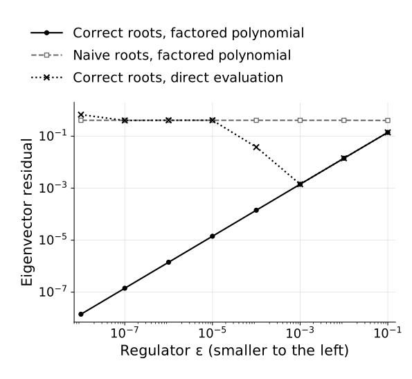
Four-site XXX eigenvector residual $r_H$ against the dimensionless regulator $\epsilon$, computed from the saved experiment with $J=1$. Factoring out the common $\epsilon^4$ preserves the correct limit; a smaller regulator alone does not ensure an accurate eigenstate. Both axes are logarithmic. The direct-evaluation curve records binary64 arithmetic in the stated environment, so its small-regulator values can vary across platforms. The finite-$\epsilon$ roots are a limiting prescription, not exact Bethe solutions.

Selected results from Python 3.9.6 and NumPy 2.0.2 are:

$\epsilon$	Correct, stable $r_H$	Correct, direct $r_H$	Naive, stable $r_H$
$10^{-2}$	$1.414\times10^{-2}$	$1.414\times10^{-2}$	$0.4082$
$10^{-4}$	$1.414\times10^{-4}$	$0.03788$	$0.4082$
$10^{-6}$	$1.414\times10^{-6}$	$0.4084$	$0.4082$
$10^{-8}$	$1.414\times10^{-8}$	$0.6710$	$0.4082$

These are dimensionless Hamiltonian residuals for $J=1$. The direct-evaluation values describe this recorded binary64 run; their detailed roundoff pattern is platform-dependent. The stable correct results are consistent with $r_H\sim\sqrt2\epsilon$, whereas the stable naive results approach $1/\sqrt6$. The saved limit and operator-identity checks use tolerance $2\times10^{-12}$; the finite-$\epsilon$ rows measure convergence and are not required to be exact eigenstates already.

In binary64 arithmetic, $2\epsilon^4$ becomes comparable to rounding in the imaginary part $1/2$ at roughly $\epsilon=10^{-4}$. At smaller values, adding $2i\epsilon^4$ to $i/2$ may lose the correction altogether. Dividing a directly computed tiny vector by $\epsilon^4$ cannot restore information already rounded away. A zero vector produced by that computation must be reported as a failed normalization, not as a zero eigenvector residual.

The saved finite-precision comparison tests these implementations. It does not replace the exact $\epsilon\to0$ calculation above, and its roundoff behavior is not an analytic error estimate for the limiting state.

Bounded extensions

Two useful follow-ups are established-result reproduction exercises. For six sites, the correction order changes with the chain length. Use

$$\lambda_1=\frac i2+\epsilon-2i\epsilon^6, \qquad \lambda_2=-\frac i2+\epsilon,$$

and take the limit of $\epsilon^{-6}B(\lambda_1)B(\lambda_2)|0\rangle$ in the polynomial convention used here. The coefficient $c=2i(-1)^{N/2}=-2i$ multiplies $\epsilon^N$; retaining the four-site $\epsilon^4$ correction would be a different prescription. Deliver a nonzero normalized state together with Hamiltonian and translation checks. The source gives the general prescription in Nepomechie and Wang 2013, v3 PDF, p. 2, equation (10), and p. 4, equation (22).

Alternatively, reproduce the four-site boundary-twist expansion through fourth order and compare the resulting normalized ray with $\chi$.

Neither exercise is presented as an open problem. A broader completeness investigation would first need a specified representation, boundary condition, admissible root classes, state-counting target, and a new literature assessment. This benchmark establishes only the finite constructions and rejections explicitly checked here.

For a bounded example of the separate counting argument, the Library proof A complete four-site XXX sector combines this singular state with a regular state and four symmetry descendants. Its six projectors sum to the sector identity; that explicit finite result does not extend the present literature assessment to general completeness questions.

References

• Nepomechie, Rafael I., and Chunguang Wang. “Algebraic Bethe ansatz for singular solutions.” Journal of Physics A: Mathematical and Theoretical 46 (2013), 325002. DOI. arXiv:1304.7978v3 PDF. All page and equation locators above refer to this PDF edition; its HTML rendering numbers some equations differently.
• Nepomechie, Rafael I., and Chunguang Wang. “Twisting singular solutions of Bethe’s equations.” Journal of Physics A: Mathematical and Theoretical 47 (2014), 505004. DOI. arXiv:1409.7382v3 PDF. The two-root parity condition and four-site twist limit are the portions used here.