A complete four-site XXX sector

When do constructed Bethe states account for every state in a sector? For a four-site periodic XXX chain with two down spins, we can answer by exhibiting six orthonormal eigenvectors. One comes from regular finite roots, one from a physical singular pair, and four from spin lowering. Their projectors sum to the identity on the six-dimensional sector. This exact example makes completeness a checkable spanning statement, rather than a count of distinct energies or a conclusion inferred from small eigenvector residuals.

Required background. Use complex inner products, orthogonal projections and the periodic XXX Hamiltonian. The regular Bethe-vector lesson defines the creation block and its root conditions. Helpful background. The singular-root benchmark derives the regulated state used below. The linear-algebra bridge reviews complete bases and degenerate eigenvalues.

Six configurations on a periodic ring

Set $N=4$, $J\gt0$, $\hbar=1$ and the lattice spacing to one. Sites are cyclic, so site $5$ means site $1$. The spin-$1/2$ Hamiltonian is

$$H=\frac J2\sum_{x=1}^{4}(I-P_{x,x+1}), \qquad S_x^\alpha=\frac12\sigma_x^\alpha.$$

The operator $P_{x,y}$ exchanges the spins at two sites. With $|0\rangle$ the all-up state, define $|x,y\rangle=S_x^-S_y^-|0\rangle$ for $x\lt y$. Exactly two spins are down, giving total $S^z=0$ and a sector $\mathcal H_2$ of dimension $\binom42=6$. Fix its orthonormal basis as

$$\mathcal B=(|12\rangle,|13\rangle,|14\rangle, |23\rangle,|24\rangle,|34\rangle).$$

Here $|12\rangle$ abbreviates $|1,2\rangle$, not a binary number. The physical bond action gives

$$\frac{H_2}{J}=\frac12 \begin{pmatrix} 2&-1&0&0&-1&0\\ -1&4&-1&-1&0&-1\\ 0&-1&2&0&-1&0\\ 0&-1&0&2&-1&0\\ -1&0&-1&-1&4&-1\\ 0&-1&0&0&-1&2 \end{pmatrix}.$$

For instance, the closing bond contributes to $H|12\rangle$:

$$H|12\rangle=J|12\rangle -\frac J2(|13\rangle+|24\rangle).$$

Active right translation increments both occupied sites, followed by cyclic reduction and reordering:

$$U|x,y\rangle=|x+1,y+1\rangle.$$

In particular, $|12\rangle\mapsto|23\rangle\mapsto|34\rangle\mapsto|14\rangle\mapsto|12\rangle$, while $|13\rangle$ and $|24\rangle$ are exchanged. The Hamiltonian is Hermitian, $U$ is unitary, and they commute. The matrices and this permutation rule provide independent checks on every state constructed below.

Spin lowering preserves energy and translation

Let $S^\alpha=\sum_xS_x^\alpha$ and $S^\pm=\sum_xS_x^\pm$ be total-spin operators. A bond swap satisfies

$$P_{x,y}(S_x^-+S_y^-)P_{x,y}=S_x^-+S_y^-.$$

It commutes with lowering operators on all other sites. Thus $[P_{x,y},S^-]=0$ for each bond and

$$[H,S^-]=0,\qquad [U,S^-]=0.$$

The second equality follows because translation merely permutes the summands of $S^-$. Consequently, a nonzero lowered vector retains its parent’s energy and translation eigenvalue. Such a vector is called a spin descendant. Its norm must still be calculated, and repeated lowering eventually gives zero.

The uniform descendant

The vacuum has energy zero and is invariant under translation. Applying $S^-$ twice gives

$$(S^-)^2|0\rangle=2\sum_{x\lt y}|x,y\rangle.$$

Each unordered pair appears twice, once in each order of the two spin flips. The squared norm is $4\times6=24$, so

$$|f\rangle=\frac{(S^-)^2|0\rangle}{2\sqrt6} =\frac1{\sqrt6}(1,1,1,1,1,1)^{\mathsf T}.$$

It obeys $H|f\rangle=0$ and $U|f\rangle=|f\rangle$. It has total spin $S=2$, inherited from the all-up state, but spin component $S^z=0$.

Three descendants of one-magnon waves

The normalized one-magnon Fourier states are

$$|k\rangle=\frac12\sum_{x=1}^{4}e^{ikx}|x\rangle, \qquad k\in\{0,\pi/2,\pi,3\pi/2\}.$$

They satisfy $H|k\rangle=J(1-\cos k)|k\rangle$ and $U|k\rangle=e^{-ik}|k\rangle$. For each nonzero allowed $k$,

$$S^+|k\rangle=\frac12\sum_xe^{ikx}|0\rangle=0, \qquad S^z|k\rangle=|k\rangle.$$

These are highest-weight states of spin one. Using $[S^+,S^-]=2S^z$ gives

$$\|S^-|k\rangle\|^2 =\langle k|(S^-S^++2S^z)|k\rangle=2.$$

Their normalized descendants are therefore

$$|d_k\rangle=\frac{S^-|k\rangle}{\sqrt2}, \qquad \langle x,y|d_k\rangle =\frac{e^{ikx}+e^{iky}}{2\sqrt2}.$$

The two terms arise because either occupied site could have carried the original down spin. The three descendants have energies $J,2J,J$ and translation eigenvalues $-i,-1,i$, respectively. Their spin remains one, while $S^z$ becomes zero.

Do not include a fourth state from $k=0$ using the same normalization. That wave is a descendant of the spin-two vacuum, and lowering it again gives the already listed $|f\rangle$. In fact $|k=0\rangle=S^-|0\rangle/2$, and $\|S^-|k=0\rangle\|^2=6$, not $2$.

Where descendants appear in the creation block

Keep the site’s polynomial normalization and monodromy order:

$$\begin{aligned} L_{ax}(u)&=(u-i/2)I+iP_{ax},\\ T_a(u)&=L_{a4}(u)\cdots L_{a1}(u) =\begin{pmatrix}A(u)&B(u)\\C(u)&D(u)\end{pmatrix}_a. \end{aligned}$$

All spectral parameters are dimensionless. Since $P_{ax}=I/2+\sum_\alpha S_x^\alpha\sigma_a^\alpha$, every factor is $uI+i\sum_\alpha S_x^\alpha\sigma_a^\alpha$. Choosing the spin term from exactly one of the four factors yields

$$T_a(u)=u^4I+iu^3\sum_\alpha S^\alpha\sigma_a^\alpha+O(u^2).$$

The upper-right entry of the spin matrix is $S^x-iS^y=S^-$. Hence

$$B(u)=iu^3S^-+O(u^2),\qquad \lim_{|u|\to\infty}\frac{B(u)}{iu^3}=S^-.$$

This is an operator-norm limit in the fixed finite-dimensional space. It explains the phrase a root at infinity: an appropriately rescaled creation block becomes global spin lowering. For a fixed regular one-magnon root $v$,

$$\lim_{|u|\to\infty} \frac{B(u)B(v)|0\rangle}{iu^3} =S^-B(v)|0\rangle.$$

Applying the operator limit twice also produces $(S^-)^2|0\rangle$. The finite values of $u$ used to take this limit need not solve the two-root Bethe equations. It is the limiting operator and the spin commutators that establish the descendant eigenstate.

The one-magnon coefficient ratio is $(v-i/2)/(v+i/2)=e^{ik}$. Thus the descendants at $k=\pi/2,\pi,3\pi/2$ come from finite creation parameters $v=-1/2,0,1/2$, respectively, followed by lowering. Their coordinate rapidities have the opposite sign; see the creation-block convention.

This expansion is Faddeev 1996, §3, equation (45), PDF. His §4, equations (98)–(105), supplies the combined auxiliary/physical spin covariance and the highest-weight property of regular on-shell Bethe vectors. Taking the auxiliary trace of that covariance gives $[\tau(u),S^-]=0$ as well. We use these symmetry statements with the explicit nonzero vectors above; they do not count states by themselves. The site’s Hamiltonian is $-J$ times Faddeev’s Hamiltonian.

Two singlets from regular and singular roots

The four descendants leave two states to find. Both will have total spin zero. On $\mathcal H_2$, where $S^z=0$, the identity

$$\mathbf S^2=S^-S^++(S^z)^2+S^z$$

shows that a vector annihilated by $S^+$ is a singlet. This can be checked directly on the following coefficient vectors.

A regular finite pair

Set $a=1/(2\sqrt3)$. The distinct roots $a,-a$ avoid $\pm i/2$ and have difference $1/\sqrt3$, so the regular two-root formulas apply. Multiplication of the actual local blocks gives

$$B(a)B(-a)|0\rangle =\frac2{27}(1,-2,1,1,-2,1)^{\mathsf T}.$$

Its squared norm is $(2/27)^2\times12=16/243$, and the normalized state is

$$|r\rangle=\frac1{\sqrt{12}} (1,-2,1,1,-2,1)^{\mathsf T}.$$

The Bethe conditions and their polynomial check are derived below. Independently of those equations, multiplying by the displayed physical matrix and applying the shift gives

$$H|r\rangle=3J|r\rangle,\qquad U|r\rangle=|r\rangle,\qquad S^+|r\rangle=0.$$

For example, the contributions to a remaining down spin at site $1$ under $S^+$ sum to $1-2+1=0$; the other three sites give the same cancellation.

The physical singular pair

The other singlet is

$$|\chi\rangle=\frac12(1,0,-1,-1,0,1)^{\mathsf T}.$$

Its four nonzero coefficients give unit norm, and the physical operators verify

$$H|\chi\rangle=J|\chi\rangle,\qquad U|\chi\rangle=-|\chi\rangle,\qquad S^+|\chi\rangle=0.$$

It is associated with the singular pair $\{i/2,-i/2\}$, but the raw vector $B(i/2)B(-i/2)|0\rangle$ is zero in our polynomial normalization. The singular-root benchmark establishes the corrected construction

$$\lim_{\epsilon\to0}\frac1{4\epsilon^4} B(i/2+\epsilon+2i\epsilon^4) B(-i/2+\epsilon)|0\rangle=|\chi\rangle.$$

The fourth-order correction changes the leading rescaled vector. A common first-order displacement alone gives the wrong limiting state.

The four-site vector and correction are treated in Nepomechie and Wang 2013, v3 HTML, §1, equations (8)–(11). Their local Lax operator divides ours by $u+i/2$, and their Hamiltonian has the opposite sign with $J=1$. The linked benchmark makes that normalization conversion explicit. Here we use the resulting state to complete a basis, without repeating the regularization calculation. The prescribed roots at finite $\epsilon$ are generally not exact roots of the untwisted Bethe equations.

An orthonormal basis, not just an energy list

The six normalized states have the following quantum numbers. The last column is total spin $S$, so $\mathbf S^2$ has eigenvalue $S(S+1)$.

State	Construction	$E/J$	$U$ eigenvalue	$S$
$\lvert f\rangle$	Twice-lowered vacuum	$0$	$1$	$2$
$\lvert d_{\pi/2}\rangle$	Lowered one-magnon wave	$1$	$-i$	$1$
$\lvert d_\pi\rangle$	Lowered one-magnon wave	$2$	$-1$	$1$
$\lvert d_{3\pi/2}\rangle$	Lowered one-magnon wave	$1$	$i$	$1$
$\lvert\chi\rangle$	Physical singular pair	$1$	$-1$	$0$
$\lvert r\rangle$	Regular finite pair	$3$	$1$	$0$

Different energies imply orthogonality because $H$ is Hermitian. The only repeated energy here is $J$, whose three listed states have distinct eigenvalues $-i,i,-1$ of the unitary operator $U$; those vectors are orthogonal too. Together with the established norms, this proves that all six vectors are orthonormal.

There are exactly six of them in a six-dimensional sector. They therefore form a complete basis of $\mathcal H_2$. If $V$ has these vectors as columns in the table’s order, then

$$\begin{aligned} V^\dagger V&=VV^\dagger=I_6,\\ V^\dagger(H_2/J)V&=\operatorname{diag}(0,1,2,1,1,3),\\ V^\dagger UV&=\operatorname{diag}(1,-i,-1,i,-1,1). \end{aligned}$$

Equivalently, the resolution of the identity is

$$I_{\mathcal H_2} =|f\rangle\langle f| +\sum_{k=\pi/2,\pi,3\pi/2}|d_k\rangle\langle d_k| +|\chi\rangle\langle\chi|+|r\rangle\langle r|.$$

This projector identity is the completeness statement. The energy spectrum, including multiplicity, is $0,J,J,J,2J,3J$. Listing just the four values $0,J,2J,3J$ would discard information about three independent states at energy $J$.

The figure makes that loss concrete. If the singular state $|\chi\rangle$ is omitted, two independent descendants still have energy $J$. All four distinct energies remain, but the retained span has only five dimensions.

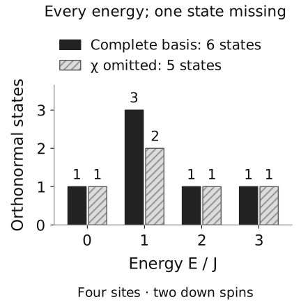
Exact state counts in the four-site, two-down-spin sector. The established orthonormal basis has multiplicities $(1,3,1,1)$ at $E/J=0,1,2,3$. Omitting $|\chi\rangle$ leaves $(1,2,1,1)$: every distinct energy survives while one independent state is missing. The bars illustrate the finite spanning argument; they are not a density of states or a proof for other chain lengths.

Reconstruct a configuration

Projecting $|12\rangle$ onto the basis gives a concrete check:

$$\begin{aligned} |12\rangle={}&\frac1{\sqrt6}|f\rangle +\frac{-1-i}{2\sqrt2}|d_{\pi/2}\rangle\\ &+\frac{-1+i}{2\sqrt2}|d_{3\pi/2}\rangle +\frac12|\chi\rangle+\frac1{\sqrt{12}}|r\rangle. \end{aligned}$$

The coefficient of $|d_\pi\rangle$ is zero. The five displayed squared moduli add to $1/6+1/4+1/4+1/4+1/12=1$. Their energy-weighted sum is $J$, agreeing with $\langle12|H|12\rangle$ in the physical matrix. A decomposition must recover the vector, its norm and its energy expectation; the last scalar alone would not prove completeness.

A finite polynomial check on the two root pairs

The preceding spanning proof does not require enumerating every solution of every version of the Bethe equations. We can nevertheless identify the two finite pairs in a compact calculation. Start with distinct finite roots $v,w$, with neither root at $\pm i/2$ and $v-w\ne\pm i$, so the regular algebraic formulas have their stated denominators. Put

$$Q(u)=(u-v)(u-w)=u^2-\sigma u+\rho, \qquad \sigma=v+w,\quad \rho=vw.$$

The regular transfer eigenvalue formula of Faddeev 1996, §4, equations (94)–(97), PDF becomes

$$\Lambda(u)=\frac{\mathcal N(u)}{Q(u)},\qquad \mathcal N(u)=(u+i/2)^4Q(u-i)+(u-i/2)^4Q(u+i).$$

At $u=v$,

$$\mathcal N(v)=-i\bigl[ (v+i/2)^4(v-w-i) -(v-i/2)^4(v-w+i)\bigr].$$

Thus $\mathcal N(v)=0$ is precisely the regular Bethe cancellation condition; the other root gives the exchanged condition. Since the roots are distinct, the two conditions are equivalent to divisibility of $\mathcal N$ by $Q$.

Reduce powers using $u^2=\sigma u-\rho$ modulo $Q$. Polynomial division gives the remainder

$$\mathcal N(u)\bmod Q(u) =-2\sigma(4\rho-\sigma^2-1)u +\frac{48\rho^2-16\rho\sigma^2-8\rho-1}{8}.$$

If $\sigma\ne0$, its linear coefficient forces $\rho=(\sigma^2+1)/4$. Substitution into the constant numerator gives $-\sigma^4$, contradicting $\sigma\ne0$. Hence $\sigma=0$, and the constant equation reduces to

$$(12\rho+1)(4\rho-1)=0.$$

The two divisible quadratics and their quotients are

$$\begin{array}{c|c} Q(u)&\mathcal N(u)/Q(u)\\ \hline u^2-1/12&2u^4+3u^2+13/8\\ u^2+1/4&2u^4+3u^2-3/8 \end{array}$$

Only the first obeys all the starting regular-root exclusions. It gives the nonzero state $|r\rangle$. The second has the singular roots $\pm i/2$: its quotient is polynomial, but its raw Bethe vector is zero. Its physical interpretation requires the separately established limiting state $|\chi\rangle$. Polynomial cancellation alone does not supply that state.

This calculation classifies the monic degree-two polynomials within the displayed divisibility problem. It neither treats repeated-root constructions nor includes roots at infinity as ordinary finite numbers. The four descendants entered by an explicit spin-lowering argument, and the complete six-state basis was proved independently.

Reproduce the finite basis checks

The XXX algebra experiment and computation notes include the actual creation-block construction and independent physical spin operators. Download the complete algebra experiment (ZIP), extract it, and run from its experiment folder:

python3 -m venv .venv
.venv/bin/python -m pip install -r requirements.txt
.venv/bin/python experiment.py --check

On Windows use python for environment creation and .venv\Scripts\python.exe for its executable. The computation notes specify supported Python versions, arithmetic, numerical norms and comparison tolerances. The four-site checks compare norms, Gram matrices, bond and shift equations, the actual regular $B$ product, and the resolution of the identity. They also remove the singular state and duplicate a retained vector deliberately: individual eigenvector equations can still pass while the spanning test fails.

Exact finite algebra establishes the result above. The executable checks test its implementation; they do not turn this six-dimensional example into a theorem for arbitrary chain length.

Check your understanding

All energies are present, but a state is missing

Delete $|\chi\rangle$ and retain the other five states. Do the retained vectors still satisfy their Hamiltonian and translation equations? Are all distinct energies still represented? Compute the missing projector and the squared norm of the retained projection of $|12\rangle$.

Solution

All five eigenvector equations remain true, and the distinct energies are still $0,J,2J,3J$: the two descendants at $k=\pi/2,3\pi/2$ retain energy $J$. But the projector sum is

$$\Pi_{\rm kept}=I_{\mathcal H_2}-|\chi\rangle\langle\chi|.$$

Its rank is five. The omitted projection of $|12\rangle$ is $|\chi\rangle/2$, with squared norm $1/4$, so $\|\Pi_{\rm kept}|12\rangle\|^2=3/4$. The Frobenius norm of $I-\Pi_{\rm kept}$ is one. Adding a duplicate retained eigenvector brings the list length back to six, but cannot increase its span: the Gram matrix becomes singular. Counting entries or distinct energies is insufficient.

Lower the zero-momentum wave

Why does the $k=0$ one-magnon wave fail to provide a new seventh vector? Calculate the lowering norm and compare its normalized descendant with $|f\rangle$.

Solution

Since $|k=0\rangle=S^-|0\rangle/2$,

$$S^-|k=0\rangle=\sum_{x\lt y}|x,y\rangle =\sqrt6|f\rangle.$$

Its squared norm is six, and the normalized descendant is exactly $|f\rangle$. The spin-one norm formula used for nonzero momenta cannot be applied: $S^+|k=0\rangle=2|0\rangle\ne0$, so that one-magnon state is not a highest weight.

References

• Faddeev, L. D. “How Algebraic Bethe Ansatz works for integrable model.” Les Houches lecture notes, 1996. Author version arXiv:hep-th/9605187v1, 26 May 1996; open PDF. Section 3, equation (45), and section 4, equations (94)–(105), supply the monodromy expansion, regular Bethe conditions and spin-symmetry framework. The explicit six-vector proof is given above.
• Nepomechie, Rafael I., and Chunguang Wang. “Algebraic Bethe ansatz for singular solutions.” Journal of Physics A: Mathematical and Theoretical 46 (32), 325002 (2013). DOI: 10.1088/1751-8113/46/32/325002. Author version arXiv:1304.7978v3; open HTML and PDF. The cited construction uses §1, equations (8)–(11), with the source normalization translated as stated above.