Build a spectral correlation sum

How do eigenstates and matrix elements determine a time-dependent observable? For one excited state of a five-site XXX chain, a local spin flip reaches just five possible one-magnon states. Summing their contributions gives an exact complex correlation function and two discrete frequency lines. You will derive the time phases, combine degenerate states without losing weight, and use two sum rules to detect missing contributions. This is a finite excited-state calculation, with no thermodynamic or ground-state approximation.

Required background. Use the normalized state and spin-flip matrix elements from Normalize states & calculate a matrix element. You need complex inner products and the one-magnon Fourier basis. Time evolution and the frequency transform are introduced below.

Helpful background. The linear algebra bridge explains orthonormal eigenbases and why degeneracy permits different basis choices.

A local spin flip in a five-site eigenstate

Keep the periodic XXX model with five sites, $J\gt0$, unit lattice spacing and $\hbar=1$:

$$H=\frac J2\sum_{x=1}^{5}(I-P_{x,x+1}), \qquad x+5\equiv x.$$

The operator $P$ swaps neighboring spins. Write $|x,y\rangle$, $x\lt y$, for two down spins in an otherwise up chain. Our normalized initial state is

$$|\Psi\rangle=\frac1{\sqrt{10}} \sum_{1\le x\lt y\le5}s_{xy}|x,y\rangle, \qquad s_{xy}=\begin{cases} -1,&y-x=1\text{ or }4,\\ +1,&y-x=2\text{ or }3. \end{cases}$$

The separation $4$ is adjacent across the closing bond. The preceding lesson obtains this state by normalizing $B(1/2)B(-1/2)|0\rangle$ and verifies $H|\Psi\rangle=2J|\Psi\rangle$ and translation eigenvalue one. The ten coefficients also give $\langle\Psi|\Psi\rangle=1$ directly.

At a fixed site $y$, let $O=S_y^+$ raise a down spin to up, and annihilate an up spin. Its adjoint is $O^\dagger=S_y^-$. The resulting one-magnon vector is

$$|g_y\rangle=O|\Psi\rangle =\frac{-|y-1\rangle-|y+1\rangle +|y-2\rangle+|y+2\rangle}{\sqrt{10}},$$

with all site labels reduced modulo five. Its squared norm is $4/10=2/5$. It is deliberately not renormalized: that norm is part of the observable’s spectral weight.

We seek the local unsymmetrized correlation

$$C_y(t)=\langle\Psi|O^\dagger(t)O|\Psi\rangle, \qquad O^\dagger(t)=e^{iHt}O^\dagger e^{-iHt}.$$

Unsymmetrized means retaining the displayed operator order without averaging it with the reversed order. That order and the sign in Heisenberg evolution fix the frequency signs. $C_y(t)$ can be complex; it is neither a transition probability nor a response commutator.

Entry check: determine the time phase

Suppose the initial energy is $2J$ and one intermediate eigenstate has energy $J$. Does its contribution carry $e^{iJt}$ or $e^{-iJt}$? Would checking only $C_y(0)$ distinguish them?

Repair: keep both energy phases

The initial bra supplies $e^{2iJt}$ and the intermediate ket supplies $e^{-iJt}$, giving $e^{iJt}$. In general the factor is $e^{-i(E_f-E_i)t}$. Both candidate signs equal one at $t=0$, so an equal-time check cannot settle the sign. Below, the first frequency moment provides an independent check.

Insert a complete basis in the reached sector

Use the five normalized one-magnon states

$$|k_m\rangle=\frac1{\sqrt5}\sum_{x=1}^{5}e^{ik_mx}|x\rangle, \qquad k_m=\frac{2\pi m}{5},\quad m=0,\ldots,4.$$

The finite geometric sum gives $\langle k_m|k_n\rangle=\delta_{mn}$. There are five such orthonormal vectors in the five-dimensional one-down-spin sector, so

$$I_{M=1}=\sum_{m=0}^{4}|k_m\rangle\langle k_m|.$$

This proves the completeness needed here. It is not a completeness claim for all Bethe states in the full spin chain. The Hamiltonian preserves this sector, and

$$H|k_m\rangle=E_m|k_m\rangle, \qquad E_m=J(1-\cos k_m).$$

Since $H|\Psi\rangle=2J|\Psi\rangle$, inserting this identity yields

$$\begin{aligned} C_y(t) &=e^{2iJt}\langle g_y|e^{-iHt}|g_y\rangle\\ &=\sum_{m=0}^{4}w_m e^{-i\Delta_m t},\\ w_m&=|\langle k_m|g_y\rangle|^2, \qquad \Delta_m=E_m-2J. \end{aligned}$$

Each contribution needs both an energy difference and a matrix-element weight. An energy list alone cannot reconstruct the correlation. This insertion of intermediate eigenstates is the finite spectral, or Lehmann, representation. Caux 2009, § II, printed pp. 3–4, equations (1)–(3), arXiv v1 PDF explains the corresponding correlation and spectral framework for a ground-state expectation. Here we have derived it for our specified excited eigenstate; the source’s ground-state restriction cannot be carried over to its allowed frequencies.

Calculate the weights and time dependence

Taking the inner product with the four terms of $|g_y\rangle$ gives

$$a_m\equiv\langle k_m|g_y\rangle =\frac{2e^{-ik_my}}{\sqrt{50}} \left(\cos2k_m-\cos k_m\right).$$

Thus $a_0=0$. At the other four allowed momenta, the cosine difference is $\pm\sqrt5/2$, so $w_m=1/10$. The site-dependent phase disappears from the weight. Consequently the local correlation is the same at each site, as translation invariance requires.

These local weights differ from the preceding lesson’s momentum-resolved weight $1/2$. The inverse transform is $S_y^+=5^{-1/2}\sum_q e^{iqy}O_q^+$; each $q$ reaches a different one-magnon state. Its factor $1/\sqrt5$ in the amplitude gives the factor $1/5$ in the weight.

Intermediate modes	$E_m/J$	$\Delta_m/J$	Weight of each state
$m=0$	$0$	$-2$	$0$
$m=1,4$	$(5-\sqrt5)/4$	$-(3+\sqrt5)/4$	$1/10$
$m=2,3$	$(5+\sqrt5)/4$	$-(3-\sqrt5)/4$	$1/10$

Combine the two states at each equal energy only after adding their weights:

$$\begin{aligned} C_y(t) &=\frac15e^{iJ(3+\sqrt5)t/4} +\frac15e^{iJ(3-\sqrt5)t/4}\\ &=\frac25e^{3iJt/4}\cos\!\left(\frac{\sqrt5Jt}{4}\right). \end{aligned}$$

At $t=0$ it equals $2/5$; at general time it need not be real. It obeys $C_y(-t)=\overline{C_y(t)}$ and $|C_y(t)|\le2/5$, as follows directly from the positive weights. This exact finite sum oscillates; it does not establish irreversible decay or a large-chain relaxation law.

Resolve the two frequency lines

Fix the time-Fourier convention

$$\mathcal S_y(\omega)=\int_{\mathbb R}e^{i\omega t}C_y(t)\,dt.$$

The transform is a distribution, since the finite correlation does not decay at large $|t|$. Using $\int e^{i(\omega-\Delta)t}dt=2\pi\delta(\omega-\Delta)$ gives

$$\mathcal S_y(\omega)=\frac{2\pi}{5} \left[ \delta\!\left(\omega+\frac{J(3+\sqrt5)}4\right) +\delta\!\left(\omega+\frac{J(3-\sqrt5)}4\right) \right].$$

Each line has integrated weight $1/5$ under $d\omega/(2\pi)$. A delta line has no ordinary finite height or width. More precisely, integrating $f(\omega)\mathcal S_y(\omega)$ with this measure gives $[f(\Delta_1)+f(\Delta_2)]/5$ for a smooth test function $f$. Here frequency has energy units because $\hbar=1$, while $\mathcal S_y$ has inverse-energy units.

Both frequencies are negative: the initial state has energy $2J$, and every intermediate state with nonzero weight has lower energy. The weights remain nonnegative. This is an excited-state local spectral measure, not the ground-state dynamical structure factor of the source and not an experimentally broadened spectrum. Reversing the Fourier sign would reverse the displayed frequencies and must be stated explicitly.

The figure connects the weighted frequency lines with the resulting real and imaginary time dependence. Its spectral stems represent integrated weights; the exact formula determines the time curves.

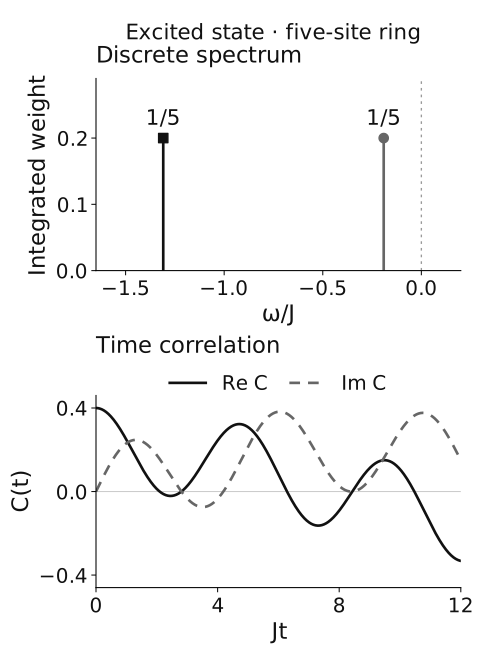
Two weighted energy differences determine this five-site excited-state correlation. The upper panel shows the lines at $\omega/J=-(3\pm\sqrt5)/4$, each with weight $1/5$ under $d\omega/(2\pi)$. The lower panel shows the real part as a solid line and the imaginary part as a dashed line for $0\le Jt\le12$. The time-Fourier convention is $e^{i\omega t}$; no line broadening is introduced. The reproducible experiment compares the exact curves with independent finite-matrix evolution.

Use two sum rules as independent checks

The zeroth moment is

$$\int\frac{d\omega}{2\pi}\mathcal S_y(\omega) =\sum_m w_m =C_y(0) =\langle\Psi|S_y^-S_y^+|\Psi\rangle =\frac25.$$

Indeed $S_y^-S_y^+=\tfrac12-S_y^z$ projects onto a down spin. A translation-invariant state with two down spins on five sites has down-spin probability $2/5$ at each site. This local equal-time value has a probability interpretation; the complex time correlation does not.

The first moment tests the energy phases as well:

$$\begin{aligned} \int\frac{d\omega}{2\pi}\omega\mathcal S_y(\omega) &=\sum_m\Delta_m w_m =-\frac{3J}{10}\\ &=\langle\Psi|O^\dagger[H,O]|\Psi\rangle =iC_y'(0). \end{aligned}$$

To check the commutator expression without the spectral table, set $y=1$. In the ordered site basis,

$$g_1=\frac1{\sqrt{10}}(0,-1,1,1,-1)^{\mathsf T}.$$

The one-magnon hopping matrix gives $\langle g_1|H|g_1\rangle=J/2$. Subtracting the initial energy times its norm gives $J/2-2J(2/5)=-3J/10$. Replacing $C_y(t)$ by its complex conjugate would pass the zeroth moment but give the opposite first moment.

Missing states, repeated energies and normalization

Keeping one state from each nonzero-energy pair gives total weight $1/5$, half the required value, although the list of distinct spectral lines looks correct. A numerical eigensolver may also choose arbitrary mixtures inside a degenerate eigenspace. Sum the weights of a complete orthonormal basis in that eigenspace; the exercise below shows why an individual basis vector’s weight is not invariant.

State normalization is a separate issue. If the initial ket is replaced by $a|\Psi\rangle$ without dividing the expectation by its squared norm, every weight and $C_y(t)$ is multiplied by $|a|^2$. A global phase has modulus one and cancels. The previous lesson’s raw Bethe vector has squared norm $5/32$, so its unnormalized equal-time expression is $1/16$, not $2/5$. Likewise, renormalizing $|g_y\rangle$ would change the observable being computed.

Reproduce the finite calculation

Download the complete correlation experiment (ZIP). Extract it, keep its two experiment folders together, and open integrable-xxx-correlations/xxx-correlations. The neighboring xxx-algebra/experiment.py supplies the actual creation-block construction used to form the initial state. Individual files are experiment.py, inputs.json, results.json, requirements.txt, and the computation notes; an individual-file download also needs the algebra companion in that sibling folder.

With Python 3.9–3.12, run from the extracted xxx-correlations folder:

python3 -m venv .venv
.venv/bin/python -m pip install -r requirements.txt
.venv/bin/python experiment.py --check

On Windows use python to create the environment and .venv\Scripts\python.exe for its executable. The computation notes specify the numerical norms, saved inputs and independent checks. The finite matrix comparison verifies this implemented example; the complete five-state Fourier basis and algebra above establish the exact finite sum.

The recorded run used Python 3.9.6, NumPy 2.0.2, $J=1$ and $y=1$. At 121 equally spaced values of $Jt$ from $0$ to $12$, evolution obtained by independently diagonalizing the bond-built one-magnon Hamiltonian agrees with the closed formula to maximum absolute complex error $1.01\times10^{-15}$, and with the Fourier spectral sum to $6.51\times10^{-16}$. These are roundoff-scale checks of a finite matrix calculation; no time-stepping approximation or frequency broadening is used.

Exercises

Guided: omit one degenerate partner

Suppose a sum retains $m=0,1,2,3$ but accidentally omits $m=4$. Find its equal-time value, first frequency moment, and difference from the complete $C_y(t)$. Does its list of distinct frequencies reveal the omission?

Hint

Subtract the omitted contribution of weight $1/10$ at $\Delta_4=-J(3+\sqrt5)/4$. Its partner $m=1$ remains at that energy.

Solution

The truncated equal-time value is $3/10$. Its first moment is

$$-\frac{3J}{10}-\frac{\Delta_4}{10} =\frac{J(-9+\sqrt5)}{40}.$$

Its correlation obeys

$$C_{\mathrm{trunc}}(t)-C_y(t) =-\frac1{10}e^{iJ(3+\sqrt5)t/4},$$

so the absolute error is $1/10$ at every time. Both distinct frequencies are still present; their weights are wrong. The equal-time sum rule catches a missing intermediate state that inspecting line locations alone misses.

Independent: rotate a degenerate eigenbasis

At $y=1$, put $k=2\pi/5$ and replace $|k\rangle,|-k\rangle$ by the normalized standing waves

$$|c\rangle=\frac{|k\rangle+|-k\rangle}{\sqrt2}, \qquad |s\rangle=\frac{|k\rangle-|-k\rangle}{i\sqrt2}.$$

Check their orthonormality and calculate their individual weights against $|g_1\rangle$. Show why the correlation remains unchanged, although neither new weight equals $1/10$.

Hint

Use $a_k=-e^{-ik}/\sqrt{10}$ and $a_{-k}=-e^{ik}/\sqrt{10}$. Conjugate the coefficient $1/i$ when taking the bra of $|s\rangle$.

Solution

The change of basis is unitary, so $\langle c|c\rangle=\langle s|s\rangle=1$ and $\langle c|s\rangle=0$. The amplitudes are

$$\langle c|g_1\rangle=-\frac{\cos k}{\sqrt5}, \qquad \langle s|g_1\rangle=-\frac{\sin k}{\sqrt5}.$$

Their squared moduli are $(3-\sqrt5)/40$ and $(5+\sqrt5)/40$, respectively. They sum to $1/5$, exactly the old pair’s total. Both vectors have the same energy, hence the same time phase; only this summed weight enters the correlation. Keeping the full degenerate eigenspace makes the result independent of the basis returned by a diagonalization routine.

Transfer: add a uniform spin-flip energy

Let $\widehat M=\sum_x(\tfrac12-S_x^z)$ count down spins and change the Hamiltonian to $H_h=H+h\widehat M$, with real $h$ in energy units. Keep the same initial state and local operator. Determine the new spectral frequencies, $C_{y,h}(t)$, and its first moment. For $h=-J$, are both lines still at negative frequencies?

Hint

The initial state has $M=2$ and each intermediate state has $M=1$. Eigenvectors and matrix-element weights stay fixed, but the two energies receive different shifts.

Solution

The initial energy becomes $2J+2h$ and the intermediate energy becomes $E_m+h$. Therefore

$$\Delta_{m,h}=\Delta_m-h, \qquad C_{y,h}(t)=e^{iht}C_y(t), \qquad \mathcal S_{y,h}(\omega)=\mathcal S_y(\omega+h).$$

Every weight is unchanged. The zeroth moment remains $2/5$, while the first is $-3J/10-2h/5$. This also follows from $[\widehat M,S_y^+]=-S_y^+$ in the commutator sum rule.

At $h=-J$ the two frequencies are $J(1-\sqrt5)/4$ and $J(1+\sqrt5)/4$: one is negative and one positive. Frequency signs reflect energy differences for the declared Hamiltonian and operator, not a universal positivity rule for an excited-state correlation.

What the finite sum establishes

You have reconstructed a complete correlation for this initial state and operator, using an explicitly complete final sector. The regular Bethe-vector lesson establishes the initial eigenstate, and the matrix-element lesson supplies its observable weights. Enlarging the chain or changing the operator may require many more intermediate states, different selection rules and controlled truncations. A thermodynamic limit requires its own analysis; neither the two-line answer nor agreement with a small matrix settles it.

References

• Caux, Jean-Sébastien. “Correlation functions of integrable models: a description of the ABACUS algorithm.” Journal of Mathematical Physics 50, 095214 (2009). DOI. Author version arXiv:0908.1660v1, submitted 12 August 2009; Open PDF. The cited printed pages and equation numbers refer to that version.