Three-site Toda: equations, invariants & evolution

Can a computation follow the open Toda chain accurately while respecting its conserved quantities? In this project you construct a three-particle trajectory, compare a time-stepping method with an independent exact representation, and measure convergence. The result is a reproducible finite-time experiment, together with an explanation of why a small conservation error alone does not establish an accurate solution or prove integrability.

Required background. Be able to derive the endpoint forces, construct the Toda Lax pair, calculate its spectral invariants, and check involution and independence. The last capability explains which analytic claims a numerical experiment cannot replace. You need elementary Python to modify the supplied experiment; its mathematical checks can also be worked by hand.

The open Toda learning sequence connects these preparations.

An open chain with three particles

Use the dimensionless open Toda model on $(q,p)\in\mathbb R^6$, with canonical brackets $\{q_i,p_j\}=\delta_{ij}$ and Hamiltonian

$$H=\frac12(p_1^2+p_2^2+p_3^2) +e^{q_1-q_2}+e^{q_2-q_3}.$$

There are two bonds, no periodic closing bond, and no forces from external endpoints. Set

$$\begin{aligned} q(0)&=(0,0,0),& p(0)&=(1,0,-1),\\ \dot q&=p,& \dot p&=F(q),\\ F(q)&=(-e_1,e_1-e_2,e_2),& e_1&=e^{q_1-q_2},\quad e_2=e^{q_2-q_3}. \end{aligned}$$

The time interval for the experiment is $0\leq t\leq6$. Positions need not remain ordered: these real canonical coordinates are not subject to a hard-core constraint.

Before writing a loop, check the initial derivatives and invariants. They must give

$$\dot q(0)=(1,0,-1),\qquad \dot p(0)=(-1,0,1).$$

The Lax matrix has diagonal $p_i$ and adjacent entries $a_i=e^{(q_i-q_{i+1})/2}$. Thus

$$L(0)=\begin{pmatrix}1&1&0\\1&0&1\\0&1&-1\end{pmatrix}, \qquad \operatorname{spec}L(0)=\{-\sqrt3,0,\sqrt3\}.$$

For $I_k=\operatorname{tr}(L^k)/k$, monitor

$$\begin{aligned} P=I_1&=p_1+p_2+p_3,\qquad I_2=H,\\ I_3&=\frac13(p_1^3+p_2^3+p_3^3) +(p_1+p_2)e_1+(p_2+p_3)e_2. \end{aligned}$$

Initially $(P,H,I_3)=(0,3,0)$. If your initial values differ, repair the Hamiltonian normalization, endpoint forces, or matrix entries before integrating. The spectral-invariants lesson supplies the trace calculation.

Advance the trajectory with velocity Verlet

For a step size $h$, first apply half a momentum kick, then a full position drift, then the remaining kick:

$$\begin{aligned} p^{n+1/2}&=p^n+\frac h2 F(q^n),\\ q^{n+1}&=q^n+h p^{n+1/2},\\ p^{n+1}&=p^{n+1/2}+\frac h2 F(q^{n+1}). \end{aligned}$$

Recalculate the force at the new position in the last line. This is the separable-Hamiltonian form of the second-order symplectic Störmer–Verlet method. Symplecticity does not mean exact conservation of this Hamiltonian at finite $h$; measure its drift. See Hairer 2010, Lecture 2, §1, Theorem 2, p. 2, PDF.

The essential implementation is short:

def force(q):
    e = np.exp(q[:-1] - q[1:])
    return np.r_[0.0, e] - np.r_[e, 0.0]

p_half = p + 0.5 * h * force(q)
q_new = q + h * p_half
p_new = p_half + 0.5 * h * force(q_new)

Because the components of $F$ sum to zero, each kick preserves total momentum in exact arithmetic. This is a useful check, but a wrong implementation with equal and opposite bond forces might also preserve momentum.

Compare with an independent reference

A closed form for the symmetric initial data

Uniqueness and reflection symmetry preserve $q=(x,0,-x)$ and $p=(v,0,-v)$. The equations reduce to $\dot x=v$, $\dot v=-e^x$, and energy conservation becomes $v^2+2e^x=3$. Define

$$\begin{aligned} s(t)&=\frac{\sqrt3}{2}t-\operatorname{artanh}\frac1{\sqrt3},\\ x(t)&=\log\frac32-2\log\cosh s(t),\\ v(t)&=-\sqrt3\tanh s(t). \end{aligned}$$

This gives $x(0)=0$, $v(0)=1$, $\dot x=v$, and

$$\dot v=-\frac32\operatorname{sech}^2s=-e^x.$$

It therefore solves the original initial-value problem, rather than merely matching the energy. It is also an independent reference: evaluating these hyperbolic functions uses neither the force routine nor a matrix eigensolver.

The reference trajectory has the following values. The remaining components are $q_2=p_2=0$, $q_3=-x$, and $p_3=-v$.

Time $t$	Position $x(t)$	Momentum $v(t)$
0	0.000000	1.000000
1	0.362695	−0.354407
2	−0.576350	−1.369711
4	−3.826786	−1.719430
6	−7.283816	−1.731654

The outer particles first approach, turn, and then separate. The central particle stays at rest by symmetry. A nonzero numerical error can coexist with exact cancellation of both $P$ and $I_3$, so this trajectory alone is insufficient for testing those diagnostics.

A QR reference that also works without symmetry

At each requested time, factor

$$e^{-tL(0)/2}=Q(t)R(t),\qquad R_{ii}(t)\gt0,$$

where $Q$ is orthogonal and $R$ is upper triangular. Then evaluate

$$L(t)=Q(t)^{\mathsf T}L(0)Q(t).$$

This factorization solution is discussed in Bloch and Karp 2023, pp. 1–2, arXiv v1 PDF. Their general symmetric matrix variable $M=-L/2$ gives the negative sign and factor $1/2$ used here. The code evaluates the exponential from the symmetric eigendecomposition of $L(0)$; it does not advance an ODE in time.

The sign can be checked directly. Set $K=Q^{\mathsf T}\dot Q$. Differentiating the factorization gives

$$-\frac12 L=K+\dot R R^{-1}.$$

Since the second term is upper triangular, $K_{i+1,i}=-a_i/2$; skew symmetry gives $K=-B$, where our $B$ has upper entries $-a_i/2$. Hence $\dot L=[L,K]=[B,L]$. The identity $L=RL(0)R^{-1}$ preserves the upper Hessenberg form; combined with symmetry this preserves tridiagonality. The adjacent entries remain positive under their Toda evolution.

Read $p_i$ from the diagonal and recover $q_i-q_{i+1}=2\log a_i$. The matrix does not record a common shift of all positions. Restore it using

$$\overline q(t)=\overline q(0)+\frac{P}{3}t, \qquad \overline q=\frac{q_1+q_2+q_3}{3}.$$

The QR formula is exact mathematically; its evaluation here uses floating-point arithmetic. At very long times the exponential becomes ill-conditioned, so this implementation is only checked over the stated short interval and the nearby points used for derivative checks.

Reproduce the experiment

Download and extract the complete Toda experiment (ZIP), then open its toda folder. The computation notes explain every norm, tolerance, and regeneration command. Individual files are also available: Python experiment, inputs, saved results, and requirements.

The recorded run used Python 3.9.6, NumPy 2.0.2, and IEEE 754 binary64 arithmetic. Use Python 3.9–3.12 for the supplied pinned environment. In the download directory, use a virtual environment:

python3 -m venv .venv
.venv/bin/python -m pip install -r requirements.txt
.venv/bin/python experiment.py --check

On Windows, use .venv\Scripts\python.exe in place of .venv/bin/python. In a repository checkout with NumPy already installed, the equivalent check is:

python3 public/computations/toda/experiment.py --check

The check recomputes the trajectories and compares them with the saved evidence; it does not rewrite the files. The last floating-point digits may vary across platforms. Use --write only when intentionally regenerating the saved results after an explained change.

The inputs also include a second case:

$$q(0)=(0.2,-0.3,0.1),\qquad p(0)=(0.7,-0.4,0.2).$$

Its initial invariants are approximately $(0.5,2.6640413167,0.4562190387)$. The unequal bonds and nonzero cubic invariant expose mistakes that the first case’s symmetry can hide. Both cases use $h=0.08,0.04,0.02,0.01$ and final time $6$.

Measure error and convergence

Let $y=(q_1,q_2,q_3,p_1,p_2,p_3)$ and define the maximum component error over every integration point in a run:

$$E(h)=\max_{0\leq nh\leq6}\; \max_{1\leq j\leq6} \left|y_j^n-y_j^{\mathrm{QR}}(nh)\right|.$$

All components are dimensionless. Use absolute invariant drift $\max_n|I_k^n-I_k^0|$, since dividing by $P(0)$ or $I_3(0)$ is meaningless in the symmetric case. Compare eigenvalues in ascending order.

The recomputed trajectory errors are:

Step $h$	Symmetric $E(h)$	Asymmetric $E(h)$
0.08	$1.240060\times10^{-3}$	$8.387314\times10^{-4}$
0.04	$3.095107\times10^{-4}$	$2.084751\times10^{-4}$
0.02	$7.734624\times10^{-5}$	$5.204395\times10^{-5}$
0.01	$1.933460\times10^{-5}$	$1.300632\times10^{-5}$

For a second-order method, $E(h)\approx Ch^2$ gives $E(h)/E(h/2)\approx4$. The measured orders $\log_2(E(h)/E(h/2))$ approach $2$: from $2.00235$ to $2.00015$ in the symmetric case and from $2.00833$ to $2.00052$ in the asymmetric case. The plot makes that shared rate visible.

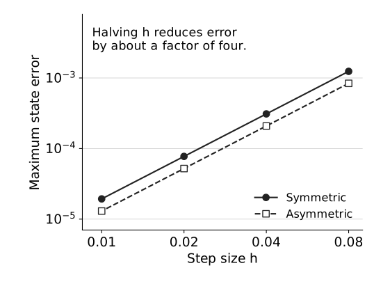
Maximum absolute error in all six position and momentum components against the QR reference over $0\leq t\leq6$, for the two initial conditions above. Both axes are logarithmic and dimensionless. Filled circles and a solid line denote the symmetric case; hollow squares and a dashed line denote the asymmetric case. These are computed values, not a schematic or a rigorous error bound.

At $h=0.01$, the symmetric run has maximum energy drift $2.70843\times10^{-5}$ and maximum eigenvalue drift $7.81856\times10^{-6}$. Its computed cubic drift is zero by symmetry. In the asymmetric run, the energy, cubic, and eigenvalue drifts are respectively $2.78245\times10^{-5}$, $1.30321\times10^{-5}$, and $1.04651\times10^{-5}$. Total-momentum drift stays below $3.3\times10^{-15}$ in all runs.

The reference is checked separately. Across the primary grids, QR and the hyperbolic closed form differ by less than $2.9\times10^{-12}$. A fourth-order centered derivative of the QR trajectory is compared with $(p,F(q))$ at $t=0,0.5,1.25,3,6$; with derivative spacing $0.005$, the largest component residual is about $1.74\times10^{-10}$ for symmetric data and $1.51\times10^{-9}$ for asymmetric data. Results at spacing $0.01$ are also retained. These derivative residuals and reference discrepancies are distinct from the Verlet discretization error.

Exercises

Guided task: check a force and a matrix entry

Write the middle force as $F_2=e^{q_1-q_2}-\square$. Complete the expression, then derive $\dot a_1$ and compute $[B,L]_{11}$. Explain how these two entries test different signs or factors. Finally, show that both Verlet kicks preserve $P$ without assuming symmetric initial data.

Independent task: assess a numerical claim

Run the experiment and produce a table of $E(h)$, maximum energy drift, and maximum cubic drift for both inputs. Report the norm, precision, final time, and observed orders. Explain why the primary case’s zero cubic drift is weak evidence. Then consider a curve $\widetilde y(t)=y(-t)$, with its momentum components left unchanged: do its conserved quantities detect that it follows the flow in the wrong time direction?

Transfer task: shift and boost the chain

Choose $c=0.4$ and $d=-0.2$. From either original exact solution form

$$q_i'(t)=q_i(t)+d+ct,\qquad p_i'(t)=p_i(t)+c.$$

Derive the transformed initial conditions, momentum, energy, cubic invariant, and Lax eigenvalues. Predict whether the QR reconstruction will recover the boost if its mean-position formula is incorrectly replaced by $\overline q(t)=0$. Test your prediction using copied experiment files so the supplied baseline remains available.

Hints and solutions

Force, matrix, and momentum checks

Hint. Differentiate the bond exponential before substituting the symmetric data. For the matrix diagonal, retain both products in the commutator.

The missing term is $e^{q_2-q_3}$. The chain rule and the first diagonal commutator entry give

$$\dot a_1=\frac12a_1(p_1-p_2),\qquad [B,L]_{11}=-\frac12a_1^2-\frac12a_1^2=-a_1^2.$$

The off-diagonal calculation tests the chain-rule factor $1/2$; the diagonal calculation tests the force direction and the sum of the two products. Since $\sum_iF_i=0$, each kick changes $\sum_i p_i$ by zero. The drift step changes no momenta. Floating-point cancellation is the only source of momentum error in this implementation of those steps.

What the numerical evidence establishes

Hint. Inspect the reduced symmetric form before interpreting $I_3=0$. A conserved value does not select a direction along a trajectory.

The energy and trajectory errors decrease under refinement as shown above. For $q=(x,0,-x)$ and $p=(v,0,-v)$, the two cubic powers and the two bond contributions cancel separately. Preserving this symmetry can therefore keep $I_3$ exactly zero while the trajectory is inaccurate. The nonsymmetric run provides the missing nonzero test.

For $\widetilde y(t)=y(-t)$, every invariant of $y$ remains constant, but $\dot{\widetilde y}=-X_H(\widetilde y)$ instead of $X_H(\widetilde y)$, where $X_H=(p,F(q))$. At $t=0$ in the primary case, the maximum component residual against the required equation is $2$. Checking the differential equations and comparing an independent trajectory catches the reversal immediately. This curve is distinct from the valid time-reversal transformation that also negates the momenta.

The calculations support the stated finite-time accuracy and second-order refinement of the implemented scheme. They do not prove involution, functional independence, or an all-time numerical error bound. The analytic three-particle integrability argument supplies the separate mathematical result.

Shift and boost

Hint. Position differences are unchanged, and adding $c$ to every momentum adds $c$ times the identity matrix to $L$.

The new initial data are $q_i'(0)=q_i(0)+d$ and $p_i'(0)=p_i(0)+c$. Because the force depends only on position differences, the transformed variables satisfy the same equations. Expanding the traces of $L'=L+c\mathbf1$ gives

$$\begin{aligned} P'&=P+3c,\\ H'&=H+cP+\frac32c^2,\\ I_3'&=I_3+2cH+c^2P+c^3,\\ \lambda_i'&=\lambda_i+c. \end{aligned}$$

For the primary initial data this gives $(P',H',I_3')=(1.2,3.24,2.464)$. The mean position is $-0.2+0.4t$. Setting it to zero would leave the reconstructed differences and Lax matrix correct while shifting every position by $0.2-0.4t$ relative to the required solution. This is another failure invisible to the spectral invariants. The supplied shift_boost_check function compares the transformed QR solution with the shifted and boosted hyperbolic solution; inspect its residuals in the saved results. When modifying the primary input, adapt its closed-form reference too.

Return to the open Toda sequence with your convergence table and explanations. You have completed the project when you can reproduce the trajectory, diagnose both symmetry and position-shift blind spots, and distinguish its numerical evidence from the analytic integrability proof.

References

• Bloch, Anthony M., and Steven N. Karp. “Symmetric Toda, gradient flows, and tridiagonalization.” arXiv:2304.10697v1 [nlin.SI], 2023. Version record; PDF. The QR representation and its symmetric matrix convention appear on pp. 1–2.
• Hairer, Ernst. Geometric Numerical Integration, Lecture 2: Symplectic integrators. TU München, January–February 2010. Author-hosted PDF. See §1, Theorem 2, p. 2 for Störmer–Verlet.